


Events in the loanable funds market can also affect the quantity of capital firms will hold. Suppose, for example, that consumers decide to increase current consumption and thus to supply fewer funds to the loanable funds market at any interest rate. This change in consumer preferences shifts the supply curve for loanable funds in Panel (a) of Figure 13.4 from S1 to S2 and raises the interest rate to r2. If there is no change in the demand for capital D1, the quantity of capital firms demand falls to K2 in Panel (b).
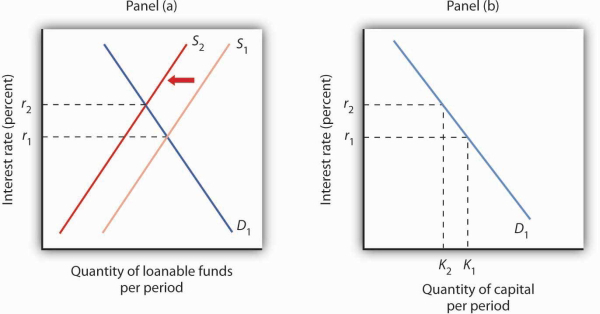
A change that begins in the loanable funds market can affect the quantity of capital firms demand. Here, a decrease in consumer saving causes a shift in the supply of loanable funds from S1 to S2 in Panel (a). Assuming there is no change in the demand for capital, the quantity of capital demanded falls from K1 to K2 in Panel (b).
Our model of the relationship between the demand for capital and the loanable funds market thus assumes that the interest rate is determined in the market for loanable funds. Given the demand curve for capital, that interest rate then determines the quantity of capital firms demand.
Table 13.7 shows that a change in the quantity of capital that firms demand can begin with a change in the demand for capital or with a change in the demand for or supply of loanable funds. A change in the demand for capital affects the demand for loanable funds and hence the interest rate in the loanable funds market. The change in the interest rate leads to a change in the quantity of capital demanded. Alternatively, a change in the loanable funds market, which leads to a change in the interest rate, causes a change in quantity of capital demanded.
|
A change originating in the capital market |
A change originating in the loanable funds market |
|
1. A change in the demand for capital leads to… |
1. A change in the demand for or supply of loanable funds leads to … |
|
2.…a change in the demand for loanable funds, which leads to… |
2.…a change in the interest rate, which leads to… |
|
3.…a change in the interest rate, which leads to… |
3.…a change in the quantity of capital demanded. |
|
4.…a change in the quantity of capital demanded. |
A change in the quantity of capital that firms demand can begin with a change in the demand for capital or with a change in the demand or supply of loanable funds.
KEY TAKEAWAYS
- The net present value (NPV) of an investment project is equal to the present value of its expected revenues minus the present value of its expected costs. Firms will want to undertake those investments for which the NPV is greater than or equal to zero.
- The demand curve for capital shows that firms demand a greater quantity of capital at lower interest rates. Among the forces that can shift the demand curve for capital are changes in expectations, changes in technology, changes in the demands for goods and services, changes in relative factor prices, and changes in tax policy.
- The interest rate is determined in the market for loanable funds. The demand curve for loanable funds has a negative slope; the supply curve has a positive slope.
- Changes in the demand for capital affect the loanable funds market, and changes in the loanable funds market affect the quantity of capital demanded.
TRY IT!
Suppose that baby boomers become increasingly concerned about whether or not the government will really have the funds to make Social Security payments to them over their retirement years. As a result, they boost saving now. How would their decisions affect the market for loanable funds and the demand curve for capital?
Case in Point: The Net Present Value of an MBA
An investment in human capital differs little from an investment in capital—one acquires an asset that will produce additional income over the life of the asset. One’s education produces—or it can be expected to produce—additional income over one’s working career.
Ronald Yeaple, a professor at the University of Rochester business school, has estimated the net present value (NPV) of an MBA obtained from each of 20 top business schools. The costs of attending each school included tuition and forgone income. To estimate the marginal revenue product of a degree, Mr. Yeaple started with survey data showing what graduates of each school were earning five years after obtaining their MBAs. He then estimated what students with the ability to attend those schools would have been earning without an MBA. The estimated marginal revenue product for each year is the difference between the salaries students earned with a degree versus what they would have earned without it. The NPV is then computed using Table 13.6.
The estimates given here show the NPV of an MBA over the first seven years of work after receiving the degree. They suggest that an MBA from 15 of the schools ranked is a good investment—but that a degree at the other schools might not be. Mr. Yeaple says that extending income projections beyond seven years would not significantly affect the analysis, because present values of projected income differentials with and without an MBA become very small.
While the Yeaple study is somewhat dated, a 2002 study by Stanford University Graduate School of Business professor Jeffrey Pfeffer and Stanford Ph.D. candidate Christina T. Fong reviewed 40 years of research on this topic and reached the conclusion that, “For the most part, there is scant evidence that the MBA credential, particularly from non-elite schools…are related to either salary or the attainment of higher level positions in organizations.”
Of course, these studies only include financial aspects of the investment and did not cover any psychic benefits that MBA recipients may incur from more interesting work or prestige.
| School | Net present value, first 7 years of work | School | Net present value, first 7 years of work |
| Harvard | $148,378 | Virginia | $30,046 |
| Chicago | 106,847 | Dartmouth | 22,509 |
| Stanford | 97,462 | Michigan | 21,502 |
| MIT | 85,736 | Carnegie-Mellon | 18,679 |
| Yale | 83,775 | Texas | 17,459 |
| Wharton | 59,486 | Rochester | −307 |
| UCLA | 55,088 | Indiana | −3,315 |
| Berkeley | 54,101 | NYU | −3,749 |
| Northwestern | 53,562 | South Carolina | −4,565 |
| Cornell | 30,874 | Duke | −17,631 |
Sources: “The MBA Cost-Benefit Analysis,” The Economist, August 6 1994, p. 58. Table reprinted with permission. Further reproduction prohibited. (We need to obtain permission to use this table again.) Jeffrey Pfeffer and Christina T. Fong, “The End of Business Schools? Less Success Than Meets the Eye,” Academy of Management Learning and Education 1:1 (September 2002): 78–95.
ANSWER TO TRY IT! PROBLEM
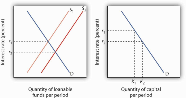
An increase in saving at each interest rate implies a rightward shift in the supply curve of loanable funds. As a result, the equilibrium interest rate falls. With the lower interest rate, there is movement downward to the right along the demand-for-capital curve, as shown.
- 10003 reads
