


Pollutants harm people and the resources they value. The marginal cost curve for a pollutant shows the additional cost imposed by each unit of the pollutant. As we saw in Figure 18.1, the marginal cost curves for all the individuals harmed by a particular pollutant are added vertically to obtain the marginal cost curve for the pollutant.
Like the marginal benefit curve for emissions, the marginal cost curve can be interpreted in two ways, as suggested in Figure 18.3. When read from left to right, the curve measures the marginal cost of additional units of emissions (MCE). If increasing the motorists’ emissions from four pounds of carbon monoxide per week to five pounds of carbon monoxide per week imposes an external cost of $2, though, the marginal benefit of not being exposed to that unit of pollutant must be $2. The marginal cost curve can thus be read from right to left as a marginal benefit curve for abating emissions (MBA). This marginal benefit curve is, in effect, the demand curve for cleaner air.
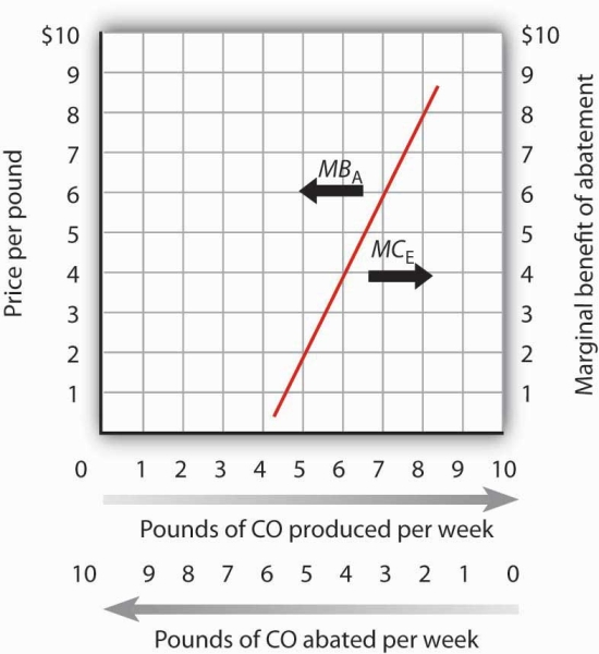
The marginal cost of the first few units of emissions is zero and then rises once emissions begin to harm people. That is the point at which the air becomes a scarce resource. Read from left to right the curve gives the marginal cost of emissions (MCE). Read from right to left, the curve gives the marginal benefit of abatement (MBA).
Economists estimate the marginal cost curve of pollution in several ways. One is to infer it from the demand for goods for which environmental quality is a complement. Another is to survey people, asking them what pollution costs—or what they would pay to reduce it. Still another is to determine the costs of damages created by pollution directly.
For example, environmental quality is a complement of housing. The demand for houses in areas with cleaner air is greater than the demand for houses in areas that are more polluted. By observing the relationship between house prices and air quality, economists can learn the value people place on cleaner air—and thus the cost of dirtier air. Studies have been conducted in cities all over the world to determine the relationship between air quality and house prices so that a measure of the demand for cleaner air can be made. They show that increased pollution levels result in lower house values.See, for example, Nir Becker and Doron Lavee, “The Benefits and Costs of Noise Reduction,” Journal of Environmental Planning and Management, 46(1) (January 2003): 97–111, which shows the negative relationship between apartment prices and noise levels (a form of pollution) in Israel.
Surveys are also used to assess the marginal cost of emissions. The fact that the marginal cost of an additional unit of emissions is the marginal benefit of avoiding the emissions suggests that surveys can be designed in two ways. Respondents can be asked how much they would be harmed by an increase in emissions, or they can be asked what they would pay for a reduction in emissions. Economists often use both kinds of questions in surveys designed to determine marginal costs.
A third kind of cost estimate is based on objects damaged by pollution. Increases in pollution, for example, require buildings to be painted more often; the increased cost of painting is one measure of the cost of added pollution.
While all of the attempts to measure cost are imperfect, the alternative is to not try to quantify cost at all. To economists, such an ostrich-like approach of sticking one’s head in the sand would be unacceptable.
- 1047 reads
