


Consider the following personal relationship that has a strong economic component: an information technology (IT) consultant and his partner, a musician, have risky incomes 1 . Each earns $5,000 in a good month and nothing in a bad month. But their risks are independent: Whether the musician has a good or bad month has no bearing on the IT consultant’s income. Individually, their incomes are quite risky, but together they are less so. Let us examine Table 7.2 to see why.
| IT Consultant | |||||
| Together | Alone | ||||
| Good | Bad | ||||
| Musician | Together | Good | $5,000; p=0.25 | $2,500; p=0.5 | $5,000; p=0.5 |
| Bad | $2,500; p=0.5 | $0; p=0.25 | $0; p=0.5 | ||
| Alone | $5,000; p=0.5 | $0; p=0.5 | |||
When the two individuals pool and subsequently split their incomes, the outcome is given in the shaded region of the table. A good month for each yields $5,000 each as before. But a good month for one, coupled with a bad month for the other, now yields $2,500 each rather than zero or $5,000. A bad month for each still yields a zero income to each.
Together, their income is more stable than when alone. To confirm this, look at the lowest row in the table. When the incomes are shared, each partner will get $5,000 one-quarter of the time (denoted by the probability p equaling 0.25), zero one-quarter of the time, and $2,500 half of the time. In contrast, when alone, they each get $5,000 and zero half of the time. The latter outcomes are more dispersed, because they are more extreme than when income is shared; the probability of extreme outcomes is greater. Another way of saying this is that the variance is greater.
As a consequence of less dispersion, the shared outcome yields more utility on average. This is because of diminishing marginal utility. In particular, if, each time one of the individuals got $2,500, they were presented with the option of getting zero half of the time and $5,000 half of the time, this latter option would make them worse off—for the simple reason that the gain in utility in going from $2,500 to $5,000 is less than the loss in utility in going to zero from $2,500. This is the consequence of diminishing MU. In general, the more stable income stream is preferred and, since the sharing option gets them closer to a more stable income stream, it yields more utility on average.
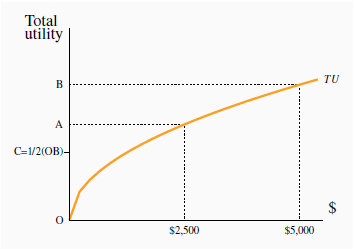
Figure 7.1 develops this argument in graphical form. It relates total utility (TU) to income. In the risky scenario, the individual gets either zero dollars or $5,000 with equal probability, and therefore gets utility of zero or OB with equal probability. Therefore, the average utility is OC (which is one half of OB, and sometimes called the ‘expected’ utility). In contrast, where no risk is involved, and the individual always gets the average payout of $2,500, utility is OA, which is greater than OC. In summary, where diminishing marginal utility exists, the average or expected utility of the event is less than the utility associated with the average or expected dollar outcome.
In this example, individuals pool their risk. But while pooling independent risks is the key to insurance, such pooling does not work when all individuals face the same risk: If the IT consultant always had a good month whenever the musician had a good month, and conversely in bad months, no change in outcomes would result from their deciding to pool their incomes.
 Risk pooling: a means of reducing risk and
increasing utility by aggregating or pooling multiple independent risks.
Risk pooling: a means of reducing risk and
increasing utility by aggregating or pooling multiple independent risks.
- 2170 reads
