


Table 10.1 tabulates the price and quantity values for a demand curve in columns 1 and 2. Column three contains the sales revenue generated at each output. It is the product of price and quantity.
Since the price denotes the revenue per unit, it is sometimes referred to as average revenue. The total revenue (TR) is plotted in Figure 10.3. It reaches a maximum at $32, where 4 units of output are produced. A greater output necessitates a lower price on every unit sold, and in this case revenue falls if the fifth unit is brought to the market. Even though the fifth unit sells for a positive price, the price on the other 4 units is now lower and the net effect is to reduce revenue. The pattern in Figure 10.3 corresponds exactly to what we examined in Measures of response: elasticities: as price is lowered from the highest possible value of $14 (where 1 unit is demanded) and the corresponding quantity increases, revenue rises, peaks, and ultimately falls as output increases. In Measures of response: elasticities we explained that this maximum revenue point occurs where the price elasticity is unity (-1), at the mid-point of a linear demand curve.
| Quantity (Q) | Price (P) | Total Revenue (TR) | Marginal Revenue (MR) | Marginal Cost (MC) | Total Cost (TC) | Profit |
| 0 | 16 | |||||
| 1 | 14 | 14 | 14 | 2 | 2 | 12 |
| 2 | 12 | 24 | 10 | 3 | 5 | 19 |
| 3 | 10 | 30 | 6 | 4 | 9 | 21 |
| 4 | 8 | 32 | 2 | 5 | 14 | 18 |
| 5 | 6 | 30 | -2 | 6 | 20 | 10 |
| 6 | 4 | 24 | -6 | 7 | 27 | -3 |
| 7 | 2 | 14 | -10 | 8 | 35 | -21 |
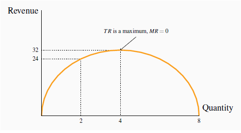
When the quantity sold increases total revenue/expenditure initially increases also. At a certain point, further sales require a price that not only increases quantity, but reduces revenue on units already being sold to such a degree that TR declines – where the demand elasticity equals - 1 (the mid point of a linear demand curve). Here the mid point occurs at Q = 4. Where the TR is a maximum the MR = 0.
Related to the total revenue function is the marginal revenue function. It is the addition to total revenue due to the sale of one more unit of the commodity.
 Marginal revenue is the change in total revenue
due to selling one more unit of the good.
Marginal revenue is the change in total revenue
due to selling one more unit of the good.
 Average revenue is the price per unit sold.
The MR in this example is defined in the fourth column of Table 10.1. When the quantity sold increases from 1 unit to 2 units total revenue increases from $14 to $24. Therefore the marginal revenue associated with the second unit of output is $10. When a third unit is sold TR increases to $30 and therefore the MR of the third unit is $6. As output increases the MR declines and eventually becomes negative – at the point where the TR is a maximum: if TR begins to decline then the additional revenue is by definition negative.
The MR function is plotted in Figure 10.4. It becomes negative when output increases from 4 to 5
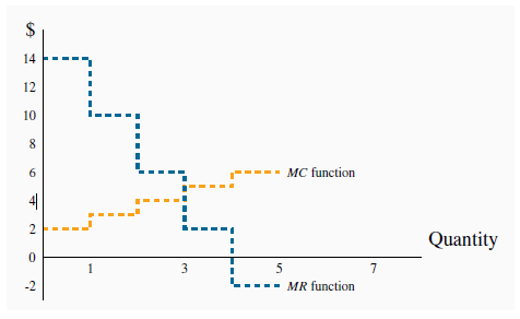
It is optimal for the monopolist to increase output as long as MR exceeds MC. In this case MR > MC for units 1, 2 and 3. But for the fourth unit MC > MR and therefore the monopolist would reduce total profit by producing it. He should produce only 3 units of output.
- 1651 reads
