


Finding the price elasticity of demand requires that we first compute percentage changes in price and in quantity demanded. We calculate those changes between two points on a demand curve.
Figure 5.1 shows a particular demand curve, a linear demand curve for public transit rides. Suppose the initial price is $0.80, and the quantity demanded is 40,000 rides per day; we are at point A on the curve. Now suppose the price falls to $0.70, and we want to report the responsiveness of the quantity demanded. We see that at the new price, the quantity demanded rises to 60,000 rides per day (point B). To compute the elasticity, we need to compute the percentage changes in price and in quantity demanded between points A and B.
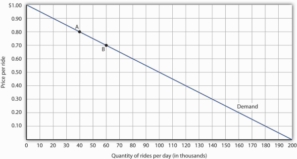
The demand curve shows how changes in price lead to changes in the quantity demanded. A movement from point A to point B shows that a $0.10 reduction in price increases the number of rides per day by 20,000. A movement from B to A is a $0.10 increase in price, which reduces quantity demanded by 20,000 rides per day.
We measure the percentage change between two points as the change in the variable divided by the average value of the variable between the two points. Thus, the percentage change in quantity between points A and B in Figure 5.1 is computed relative to the average of the quantity values at points A and B: (60,000 + 40,000)/2 = 50,000. The percentage change in quantity, then, is 20,000/50,000, or 40%. Likewise, the percentage change in price between points A and B is based on the average of the two prices: ($0.80 + $0.70)/2 = $0.75, and so we have a percentage change of −0.10/0.75, or −13.33%. The price elasticity of demand between points A and B is thus 40%/(−13.33%) = −3.00.
This measure of elasticity, which is based on percentage changes relative to the average value of each variable between two points, is called arc elasticity. The arc elasticity method has the advantage that it yields the same elasticity whether we go from point A to point B or from point B to point A. It is the method we shall use to compute elasticity.
For the arc elasticity method, we calculate the price elasticity of demand using the average value of price, P¯, and the average value of quantity demanded, Q¯. We shall use the Greek letter Δ to mean “change in,” so the change in quantity between two points is ΔQ and the change in price is ΔP. Now we can write the formula for the price elasticity of demand as
| eD = ΔQ/Q¯ΔP/P¯ |
The price elasticity of demand between points A and B is thus:
eD = 20,000(40,000 + 60,000)/2-$0.10($0.80 + $0.70)/2=40%-13.33%=-3.00
With the arc elasticity formula, the elasticity is the same whether we move from point A to point B or from point B to point A. If we start at point B and move to point A, we have:
eD = -20,000(60,000 + 40,000)/20.10($0.70 + $0.80)/2 = -40%13.33% = -3.00
The arc elasticity method gives us an estimate of elasticity. It gives the value of elasticity at the midpoint over a range of change, such as the movement between points A and B. For a precise computation of elasticity, we would need to consider the response of a dependent variable to an extremely small change in an independent variable. The fact that arc elasticities are approximate suggests an important practical rule in calculating arc elasticities: we should consider only small changes in independent variables. We cannot apply the concept of arc elasticity to large changes.
Another argument for considering only small changes in computing price elasticities of demand will become evident in the next section. We will investigate what happens to price elasticities as we move from one point to another along a linear demand curve.
Heads Up!
Notice that in the arc elasticity formula, the method for computing a percentage change differs from the standard method with which you may be familiar. That method measures the percentage change in a variable relative to its original value. For example, using the standard method, when we go from point A to point B, we would compute the percentage change in quantity as 20,000/40,000 = 50%. The percentage change in price would be −$0.10/$0.80 = −12.5%. The price elasticity of demand would then be 50%/(−12.5%) = −4.00. Going from point B to point A, however, would yield a different elasticity. The percentage change in quantity would be −20,000/60,000, or −33.33%. The percentage change in price would be $0.10/$0.70 = 14.29%. The price elasticity of demand would thus be −33.33%/14.29% = −2.33. By using the average quantity and average price to calculate percentage changes, the arc elasticity approach avoids the necessity to specify the direction of the change and, thereby, gives us the same answer whether we go from A to B or from B to A.
- 2182 reads
