


If you know a person's pinky (smallest) finger length, do you think you could predict that person's height? Collect data from your class (pinky finger length, in inches). The independent variable, x, is pinky finger length and the dependent variable, y, is height.
For each set of data, plot the points on graph paper. Make your graph big enough and use a ruler. Then "by eye" draw a line that appears to "fit" the data. For your line, pick two convenient points and use them to find the slope of the line. Find the y-intercept of the line by extending your lines so they cross the y-axis. Using the slopes and the y-intercepts, write your equation of "best fit". Do you think everyone will have the same equation? Why or why not?
Using your equation, what is the predicted height for a pinky length of 2.5 inches?
Example 6.6
A random sample of 11 statistics students produced the following data where x is the third exam score, out of 80, and y is the final exam score, out of 200. Can you predict the final exam score of a random student if you know the third exam score?
|
x (third exam score) |
y (fnal exam score) |
|---|---|
|
65 |
175 |
|
67 |
133 |
|
71 |
185 |
|
71 |
163 |
|
66 |
126 |
|
75 |
198 |
|
67 |
153 |
|
70 |
163 |
|
71 |
159 |
|
69 |
151 |
|
69 |
159 |
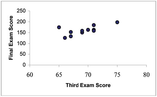
The third exam score, x, is the independent variable and the final exam score, y, is the dependent variable. We will plot a regression line that best "fits" the data. If each of you were to fit
a line "by eye", you would draw different lines. We can use what is called a least-squares regression line to obtain the best fit line. Consider the following
diagram. Each point of data is of the form (x, y) and each point of the line of best fit using least-squares linear regression has the form (x,  ).
).
The  is read "y hat" and is
the estimated value of y. It is the value of y obtained using the regression line. It is not generally equal to y from data.
is read "y hat" and is
the estimated value of y. It is the value of y obtained using the regression line. It is not generally equal to y from data.
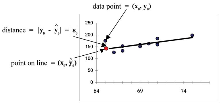
The term  is called the "error" or residual. It is not an error in the sense of a mistake. The absolute value of a residual measures the vertical distance between the actual value
of y and the estimated value of y. In other words, it measures the vertical distance between the actual data point and the predicted point on the line.
is called the "error" or residual. It is not an error in the sense of a mistake. The absolute value of a residual measures the vertical distance between the actual value
of y and the estimated value of y. In other words, it measures the vertical distance between the actual data point and the predicted point on the line.
If the observed data point lies above the line, the residual is positive, and the line underestimates the actual data value for y. If the observed data point lies below the line, the residual is negative, and the line overestimates that actual data value for y.
 is the residual
for the point shown. Here the point lies above the line and the residual is positive.
is the residual
for the point shown. Here the point lies above the line and the residual is positive.
 = the Greek letter epsilon
For each data point, you can calculate the residuals or errors, 
Each  is a vertical distance.
For the example about the third exam scores and the fnal exam scores for the 11 statistics students, there are 11 data points. Therefore, there are 11  values. If you square each
  and add, you get
This is called the Sum of Squared Errors (SSE).
Using calculus, you can determine the values of a and b that make the SSE a minimum. When you make the SSE a minimum, you have determined the points that are on the line of best fit. It turns out that the line of best fit has the equation:

where  and
and
 and
and  are the sample means of the x values and the y values, respectively. The best fit line
always passes through the point (
are the sample means of the x values and the y values, respectively. The best fit line
always passes through the point ( ,
,  ).
).
The slope b can be written as  where sy = the standard deviation of the y values and sx the standard
deviation of the x values. r is the correlation coefficient which is discussed in the next section.
where sy = the standard deviation of the y values and sx the standard
deviation of the x values. r is the correlation coefficient which is discussed in the next section.
Least Squares Criteria for Best Fit
The process of fitting the best fit line is called linear regression. The idea behind finding the best fit line is based on the assumption that the data are scattered about a straight line. The criteria for the best fit line is that the sum of the squared errors (SSE) is minimized, that is made as small as possible. Any other line you might choose would have a higher SSE than the best fit line. This best fit line is called the least squares regression line.
THIRD EXAM vs FINAL EXAM EXAMPLE:
The graph of the line of best fit for the third exam/final exam example is shown below:
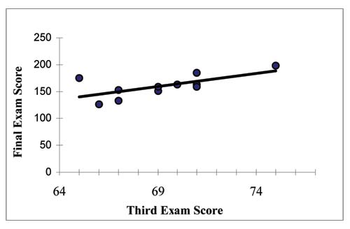
The least squares regression line (best fit line) for the third exam/final exam example has the equation:
Remember, it is always important to plot a scatter diagram first. If the scatter plot indicates that there is a linear relationship between the variables, then it is reasonable to use a best fit line to make predictions for y given x within the domain of x-values in the sample data, but not necessarily for x-values outside that domain.
You could use the line to predict the final exam score for a student who earned a grade of 73 on the third exam.
You should NOT use the line to predict the final exam score for a student who earned a grade of 50 on the third exam, because 50 is not within the domain of the x-values in the sample data, which are between 65 and 75.
UNDERSTANDING SLOPE
The slope of the line, b, describes how changes in the variables are related. It is important to interpret the slope of the line in the context of the situation represented by the data. You should be able to write a sentence interpreting the slope in plain English.
INTERPRETATION OF THE SLOPE: The slope of the best fit line tells us how the dependent variable (y) changes for every one unit increase in the independent (x) variable, on average.
THIRD EXAM vs FINAL EXAM EXAMPLE
Slope: The slope of the line is b 4.83.
Interpretation: For a one point increase in the score on the third exam, the fnal exam score increases by 4.83 points, on average.
- 2078 reads
