


To construct a production possibilities curve, we will begin with the case of a hypothetical firm, Alpine Sports, Inc., a specialized sports equipment manufacturer. Christie Ryder began the business 15 years ago with a single ski production facility near Killington ski resort in central Vermont. Ski sales grew, and she also saw demand for snowboards rising—particularly after snowboard competition events were included in the 2002 Winter Olympics in Salt Lake City. She added a second plant in a nearby town. The second plant, while smaller than the first, was designed to produce snowboards as well as skis. She also modified the first plant so that it could produce both snowboards and skis. Two years later she added a third plant in another town. While even smaller than the second plant, the third was primarily designed for snowboard production but could also produce skis.
We can think of each of Ms. Ryder’s three plants as a miniature economy and analyze them using the production possibilities model. We assume that the factors of production and technology available to each of the plants operated by Alpine Sports are unchanged.
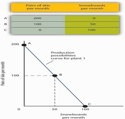
Suppose the first plant, Plant 1, can produce 200 pairs of skis per month when it produces only skis. When devoted solely to snowboards, it produces 100 snowboards per month. It can produce skis and snowboards simultaneously as well.
The table in Figure 2.1 gives three combinations of skis and snowboards that Plant 1 can produce each month. Combination A involves devoting the plant entirely to ski production; combination C means shifting all of the plant’s resources to snowboard production; combination B involves the production of both goods. These values are plotted in a production possibilities curve for Plant 1. The curve is a downward-sloping straight line, indicating that there is a linear, negative relationship between the production of the two goods.
Neither skis nor snowboards is an independent or a dependent variable in the production possibilities model; we can assign either one to the vertical or to the horizontal axis. Here, we have placed the number of pairs of skis produced per month on the vertical axis and the number of snowboards produced per month on the horizontal axis.
The negative slope of the production possibilities curve reflects the scarcity of the plant’s capital and labor. Producing more snowboards requires shifting resources out of ski production and thus producing fewer skis. Producing more skis requires shifting resources out of snowboard production and thus producing fewer snowboards.
The slope of Plant 1’s production possibilities curve measures the rate at which Alpine Sports must give up ski production to produce additional snowboards. Because the production possibilities curve for Plant 1 is linear, we can compute the slope between any two points on the curve and get the same result. Between points A and B, for example, the slope equals −2 pairs of skis/snowboard (equals −100 pairs of skis/50 snowboards). (Many students are helped when told to read this result as “−2 pairs of skis per snowboard.”) We get the same value between points B and C, and between points A and C.
The Figure 2.1 shows the combinations of pairs of skis and snowboards that Plant 1 is capable of producing each month.
These are also illustrated with a production possibilities curve. Notice that this curve is linear.
To see this relationship more clearly, examine Figure 2.2. Suppose Plant 1 is producing 100 pairs of skis and 50 snowboards per month at point B. Now consider what would happen if Ms. Ryder decided to produce 1 more snowboard per month. The segment of the curve around point B is magnified in Figure 2.2. The slope between points B and B′ is −2 pairs of skis/snowboard. Producing 1 additional snowboard at point B′ requires giving up 2 pairs of skis. We can think of this as the opportunity cost of producing an additional snowboard at Plant 1. This opportunity cost equals the absolute value of the slope of the production possibilities curve.
The slope of the linear production possibilities curve in the following Figure 2.2 is constant; it is −2 pairs of skis/snowboard. In the section of the curve shown here, the slope can be calculated between points B and B′. Expanding snowboard production to 51 snowboards per month from 50 snowboards per month requires a reduction in ski production to 98 pairs of skis per month from 100 pairs. The slope equals −2 pairs of skis/snowboard (that is, it must give up two pairs of skis to free up the resources necessary to produce one additional snowboard). To shift from B′ to B″, Alpine Sports must give up two more pairs of skis per snowboard. The absolute value of the slope of a production possibilities curve measures the opportunity cost of an additional unit of the good on the horizontal axis measured in terms of the quantity of the good on the vertical axis that must be forgone.
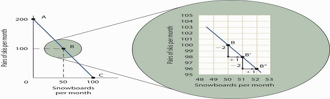
The absolute value of the slope of any production possibilities curve equals the opportunity cost of an additional unit of the good on the horizontal axis. It is the amount of the good on the vertical axis that must be given up in order to free up the resources required to produce one more unit of the good on the horizontal axis. We will make use of this important fact as we continue our investigation of the production possibilities curve.
Figure 2.3 shows production possibilities curves for each of the firm’s three plants. Each of the plants, if devoted entirely to snowboards, could produce 100 snowboards. Plants 2 and 3, if devoted exclusively to ski production, can produce 100 and 50 pairs of skis per month, respectively. The exhibit gives the slopes of the production possibilities curves for each plant. The opportunity cost of an additional snowboard at each plant equals the absolute values of these slopes (that is, the number of pairs of skis that must be given up per snowboard).
The slopes of the production possibilities curves for each plant differ. The steeper the curve, the greater the opportunity cost of an additional snowboard. Here, the opportunity cost is lowest at Plant 3 and greatest at Plant 1.
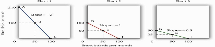
The exhibit gives the slopes of the production possibilities curves for each of the firm’s three plants. The opportunity cost of an additional snowboard at each plant equals the absolute values of these slopes. More generally, the absolute value of the slope of any production possibilities curve at any point gives the opportunity cost of an additional unit of the good on the horizontal axis, measured in terms of the number of units of the good on the vertical axis that must be forgone.
The greater the absolute value of the slope of the production possibilities curve, the greater the opportunity cost will be. The plant for which the opportunity cost of an additional snowboard is greatest is the plant with the steepest production possibilities curve; the plant for which the opportunity cost is lowest is the plant with the flattest production possibilities curve. The plant with the lowest opportunity cost of producing snowboards is Plant 3; its slope of −0.5 means that Ms. Ryder must give up half a pair of skis in that plant to produce an additional snowboard. In Plant 2, she must give up one pair of skis to gain one more snowboard. We have already seen that an additional snowboard requires giving up two pairs of skis in Plant 1.
- 4461 reads
