


To illustrate how we will use the model of aggregate demand and aggregate supply, let us examine the impact of two events: an increase in the cost of health care and an increase in government purchases. The first reduces short-run aggregate supply; the second increases aggregate demand. Both events change equilibrium real GDP and the price level in the short run.
A Change in the Cost of Health Care
In the United States, most people receive health insurance for themselves and their families through their employers. In fact, it is quite common for employers to pay a large percentage of employees’ health insurance premiums, and this benefit is often written into labor contracts. As the cost of health care has gone up over time, firms have had to pay higher and higher health insurance premiums. With nominal wages fixed in the short run, an increase in health insurance premiums paid by firms raises the cost of employing each worker. It affects the cost of production in the same way that higher wages would. The result of higher health insurance premiums is that firms will choose to employ fewer workers.
Suppose the economy is operating initially at the short-run equilibrium at the intersection of AD1 and SRAS1, with a real GDP of Y1 and a price level of P1, as shown in Figure 22.7. This is the initial equilibrium price and output in the short run. The increase in labor cost shifts the short-run aggregate supply curve to SRAS2. The price level rises to P2 and real GDP falls to Y2.
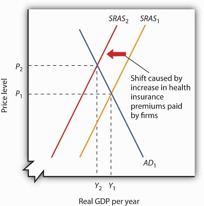
An increase in health insurance premiums paid by firms increases labor costs, reducing short-run aggregate supply from SRAS1 to SRAS2. The price level rises from P1 to P2 and output falls from Y1 to Y2.
A reduction in health insurance premiums would have the opposite effect. There would be a shift to the right in the short-run aggregate supply curve with pressure on the price level to fall and real GDP to rise.
A Change in Government Purchases
Suppose the federal government increases its spending for highway construction. This circumstance leads to an increase in U.S. government purchases and an increase in aggregate demand.
Assuming no other changes affect aggregate demand, the increase in government purchases shifts the aggregate demand curve by a multiplied amount of the initial increase in government purchases to AD2 in Figure 22.8. Real GDP rises from Y1 to Y2, while the price level rises from P1 to P2. Notice that the increase in real GDP is less than it would have been if the price level had not risen.
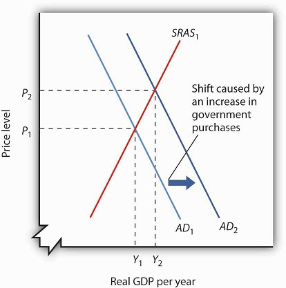
An increase in government purchases boosts aggregate demand from AD1 to AD2. Short-run equilibrium is at the intersection of AD2 and the short-run aggregate supply curve SRAS1. The price level rises to P2 and real GDP rises to Y2.
In contrast, a reduction in government purchases would reduce aggregate demand. The aggregate demand curve shifts to the left, putting pressure on both the price level and real GDP to fall.
In the short run, real GDP and the price level are determined by the intersection of the aggregate demand and short-run aggregate supply curves. Recall, however, that the short run is a period in which sticky prices may prevent the economy from reaching its natural level of employment and potential output. In the next section, we will see how the model adjusts to move the economy to long-run equilibrium and what, if anything, can be done to steer the economy toward the natural level of employment and potential output.
KEY TAKEAWAYS
- The short run in macroeconomics is a period in which wages and some other prices are sticky. The long run is a period in which full wage and price flexibility, and market adjustment, has been achieved, so that the economy is at the natural level of employment and potential output.
- The long-run aggregate supply curve is a vertical line at the potential level of output. The intersection of the economy’s aggregate demand and long-run aggregate supply curves determines its equilibrium real GDP and price level in the long run.
- The short-run aggregate supply curve is an upward-sloping curve that shows the quantity of total output that will be produced at each price level in the short run. Wage and price stickiness account for the shortrun aggregate supply curve’s upward slope.
- Changes in prices of factors of production shift the short-run aggregate supply curve. In addition, changes in the capital stock, the stock of natural resources, and the level of technology can also cause the short-run aggregate supply curve to shift.
- In the short run, the equilibrium price level and the equilibrium level of total output are determined by the intersection of the aggregate demand and the short-run aggregate supply curves. In the short run, output can be either below or above potential output.
TRY IT!
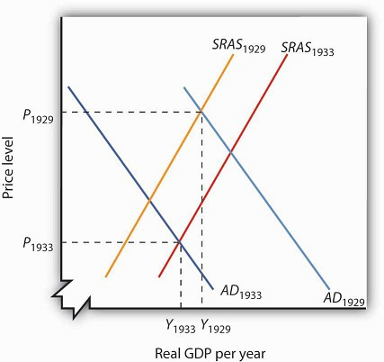
The tools we have covered in this section can be used to understand the Great Depression of the 1930s. We know that investment and consumption began falling in late 1929. The reductions were reinforced by plunges in net exports and government purchases over the next four years. In addition, nominal wages plunged 26% between 1929 and 1933. We also know that real GDP in 1933 was 30% below real GDP in 1929. Use the tools of aggregate demand and short-run aggregate supply to graph and explain what happened to the economy between 1929 and 1933.
Case in Point: The U.S. Recession of 2001
What were the causes of the U.S. recession of 2001? Economist Kevin Kliesen of the Federal Reserve Bank of St.Louis points to four factors that, taken together, shifted the aggregate demand
curve to the left and kept it there for a long enough period to keep real GDP falling for about nine months. They were the fall in stock market prices, the decrease in business investment
both for computers and software and in structures, the decline in the real value of exports, and the aftermath of 9/11. Notable exceptions to this list of culprits were the behavior of
consumer spending during the period and new residential housing, which falls into the investment category.
During the expansion in the late 1990s, a surging stock market probably made it easier for firms to raise funding for investment in both structures and information technology. Even though the
stock market bubble burst well before the actual recession, the continuation of projects already underway delayed the decline in the investment component of GDP. Also, spending for
information technology was probably prolonged as firms dealt with Y2K computing issues, that is, computer problems associated with the change in the date from 1999 to 2000. Most computers
used only two digits to indicate the year, and when the year changed from ’99 to ’00, computers did not know how to interpret the change, and extensive reprogramming of computers was
required.
Real exports fell during the recession because (1) the dollar was strong during the period and (2) real GDP growth in the rest of the world fell almost 5% from 2000 to 2001.
Then, the terrorist attacks of 9/11, which literally shut down transportation and financial markets for several days, may have prolonged these negative tendencies just long enough to turn
what might otherwise have been a mild decline into enough of a downtown to qualify the period as a recession.
During this period the measured price level was essentially stable—with the implicit price deflator rising by less than 1%. Thus, while the aggregate demand curve shifted left as a result of
all the reasons given above, there was also a leftward shift in the short-run aggregate supply curve.
Source: Kevin L. Kliesen, “The 2001 Recession: How Was It Different and What Developments May Have Caused It?” The Federal Reserve Bank of St. Louis Review, September/October 2003:
23–37.
ANSWER TO TRY IT! PROBLEM
All components of aggregate demand (consumption, investment, government purchases, and net exports) declined between 1929 and 1933. Thus the aggregate demand curve shifted markedly to the
left, moving from AD1929 to AD1933. The reduction in nominal wages corresponds to an increase in short-run aggregate supply from SRAS1929 to SRAS1933. Since real GDP in 1933 was less than
real GDP in 1929, we know that the movement in the aggregate demand curve was greater than that of the short-run aggregate supply curve.
- 11996 reads
