


The stability of velocity in the long run underlies the close relationship we have seen between changes in the money supply and changes in the price level. But velocity is not stable in the short run; it varies significantly from one period to the next. Figure 26.6 shows annual values of the velocity of M2 from 1960 through 2007. Velocity is quite variable, so other factors must affect economic activity. Any change in velocity implies a change in the demand for money. For analyzing the effects of monetary policy from one period to the next, we apply the framework that emphasizes the impact of changes in the money market on aggregate demand.
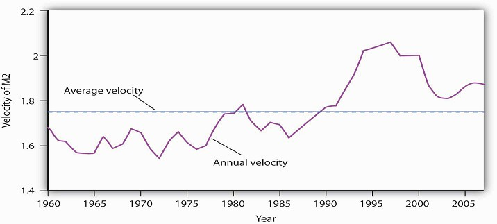
Source: Survey of Current Business, Oct. 2006; Federal Reserve Statistical Release Nov. 9, 2006, Table H-6; Economic Report of the President, 2009, Tables B-1 and B-69.
The factors that cause velocity to fluctuate are those that influence the demand for money, such as the interest rate and expectations about bond prices and future price levels. We can gain some insight about the demand for money and its significance by rearranging terms in the equation of exchange so that we turn the equation of exchange into an equation for the demand for money. If we multiply both sides of Equation 26.1 by the reciprocal of velocity, 1/V, we have this equation for money demand:
EQUATION 26.10
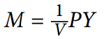
The equation of exchange can thus be rewritten as an equation that expresses the demand for money as a percentage, given by 1/V, of nominal GDP. With a velocity of 1.87, for example, people wish to hold a quantity of money equal to 53.4% (1/1.87) of nominal GDP. Other things unchanged, an increase in money demand reduces velocity, and a decrease in money demand increases velocity.
If people wanted to hold a quantity of money equal to a larger percentage of nominal GDP, perhaps because interest rates were low, velocity would be a smaller number. Suppose, for example, that people held a quantity of money equal to 80% of nominal GDP. That would imply a velocity of 1.25. If people held a quantity of money equal to a smaller fraction of nominal GDP, perhaps owing to high interest rates, velocity would be a larger number. If people held a quantity of money equal to 25% of nominal GDP, for example, the velocity would be 4.
As another example, in the chapter on financial markets and the economy, we learned that money demand falls when people expect inflation to increase. In essence, they do not want to hold money that they believe will only lose value, so they turn it over faster, that is, velocity rises. Expectations of deflation lower the velocity of money, as people hold onto money because they expect it will rise in value.
In our first look at the equation of exchange, we noted some remarkable conclusions that would hold if velocity were constant: a given percentage change in the money supply M would produce an equal percentage change in nominal GDP, and no change in nominal GDP could occur without an equal percentage change in M. We have learned, however, that velocity varies in the short run. Thus, the conclusions that would apply if velocity were constant must be changed.
First, we do not expect a given percentage change in the money supply to produce an equal percentage change in nominal GDP. Suppose, for example, that the money supply increases by 10%. Interest rates drop, and the quantity of money demanded goes up. Velocity is likely to decline, though not by as large a percentage as the money supply increases. The result will be a reduction in the degree to which a given percentage increase in the money supply boosts nominal GDP.
Second, nominal GDP could change even when there is no change in the money supply. Suppose government purchases increase. Such an increase shifts the aggregate demand curve to the right, increasing real GDP and the price level. That effect would be impossible if velocity were constant. The fact that velocity varies, and varies positively with the interest rate, suggests that an increase in government purchases could boost aggregate demand and nominal GDP. To finance increased spending, the government borrows money by selling bonds. An increased supply of bonds lowers their price, and that means higher interest rates. The higher interest rates produce the increase in velocity that must occur if increased government purchases are to boost the price level and real GDP.
Just as we cannot assume that velocity is constant when we look at macroeconomic behavior period to period, neither can we assume that output is at potential. With both V and Y in the equation of exchange variable, in the short run, the impact of a change in the money supply on the price level depends on the degree to which velocity and real GDP change.
In the short run, it is not reasonable to assume that velocity and output are constants. Using the model in which interest rates and other factors affect the quantity of money demanded seems more fruitful for understanding the impact of monetary policy on economic activity in that period. However,the empirical evidence on the long-run relationship between changes in money supply and changes in the price level that we presented earlier gives us reason to pause. As Federal Reserve Governor from 1996 to 2002 Laurence H. Meyer put it: “I believe monitoring money growth has value, even for central banks that follow a disciplined strategy of adjusting their policy rate to ongoing economic developments. The value may be particularly important at the extremes: during periods of very high inflation, as in the late 1970s and early 1980s in the United States … and in deflationary episodes.”[5]
It would be a mistake to allow short-term fluctuations in velocity and output to lead policy makers to completely ignore the relationship between money and price level changes in the long run.
KEY TAKEAWAYS
- The equation of exchange can be written MV = PY.
- When M, V, P, and Y are changing, then %ΔM + %ΔV = %ΔP + %ΔY, where Δ means “change in.”
- In the long run, V is constant, so %ΔV = 0. Furthermore, in the long run Y tends toward YP, so %ΔM = %ΔP.
- In the short run, V is not constant, so changes in the money supply can affect the level of income.
TRY IT!
The Case in Point on velocity in the Confederacy during the Civil War shows that, assuming real GDP in the South was constant, velocity rose. What happened to money demand? Why did it change?
Case in Point: Velocity and the Confederacy
The Union and the Confederacy financed their respective efforts during the Civil War largely through the issue of paper money. The Union roughly doubled its money supply through this process,
and the Confederacy printed enough “Confederates” to increase the money supply in the South 20-fold from 1861 to 1865. That huge increase in the money supply boosted the price level in the
Confederacy dramatically. It rose from an index of 100 in 1861 to 9,200 in 1865.
Estimates of real GDP in the South during the Civil War are unavailable, but it could hardly have increased very much. Although production undoubtedly rose early in the period, the South lost
considerable capital and an appalling number of men killed in battle. Let us suppose that real GDP over the entire period remained constant. For the price level to rise 92-fold with a 20-fold
increase in the money supply, there must have been a 4.6-fold increase in velocity. People in the South must have reduced their demand for Confederates.
An account of an exchange for eggs in 1864 from the diary of Mary Chestnut illustrates how eager people in the South were to part with their Confederate money. It also suggests that other
commodities had assumed much greater relative value:
“She asked me 20 dollars for five dozen eggs and then said she would take it in “Confederate.” Then I would have given her 100 dollars as easily. But if she had taken my offer of yarn! I
haggle in yarn for the millionth part of a thread! … When they ask for Confederate money, I never stop to chafer [bargain or argue]. I give them 20 or 50 dollars cheerfully for
anything.”
sources: C. Vann Woodward, ed., Mary Chestnut’s Civil War (New Haven, CT: Yale University Press, 1981), 749. Money and price data from E. M.
Lerner, “Money, Prices, and Wages in the Confederacy, 1861–1865,” Journal of Political Economy 63 (February 1955): 20–40.
ANSWER TO TRY IT! PROBLEM
People in the South must have reduced their demand for money. The fall in money demand was probably due to the expectation that the price level would continue to rise. In periods of high inflation, people try to get rid of money quickly because it loses value rapidly.
- 2602 reads
