


This section introduces the techniques used to model the financial market with uncertainties. We will start from the very basic model. To start, we consider a market with M assets. There are two things we need to define:
- For all possible outcomes of the future market, we define
Ω = the set of events coming from the market histories. (2.1)
-
For each asset 1 £ i £ M with future market ω outcome and future time t ≥ 0, we define
St(i) (ω) = the price of asset i at time t. (2.2)
We demonstrate the use of the modelling technique by considering two different forms of models:
- the single-period market model; and
- the two-period market model.
The single-period market model
This model is only concerned with one asset, one
period and two possible market outcomes. This model is commonly called the binomial model.
We
assume t = 0 at the beginning (today), and t = 1 at the end of the period.
There are two possible outcomes at the first period, we need to define the following variables for the
model:
- market upswing, denoted by u, and the asset return denoted by g, or
-
market downswing, denoted by d, and the asset return denoted by l.
Intuitively, we have 1 < g. Mathematically, we define the event space of a single-period model as
 and the price of the assets at t
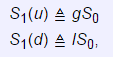 where S0 is the price of the assets at t = 0.
If we work this one model period further, we derive the second model.
The two-period market model
This model extends the one period mode that is concerned with one asset over two periods.
Starting with the first period, we have another two possible outcomes at the second period, i.e. a market upswing, denoted by u, and with the asset return denoted by g; or a market downswing , denoted by d, and with the asset return denoted by l.
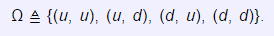
In this situation, we have 22 = 4 possible events, which is given as
As usual, the price of the assets at t = 1 and t = 2 is given by
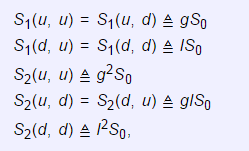
where S0 is the price of the assets t = 0.
Having discussed the single-period and the two-period models, we can now use the same approach to generalize a standard form of the equation. We define

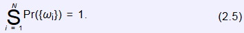
For each ωi Î Ω, we have

and
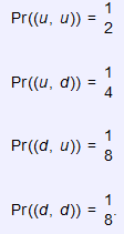
The following example demonstrates how the probabilities are included in the two-period binomial market model. The set of market histories is given as

The following observation is made:
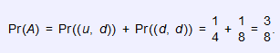
Let A be the event of downswing in the second period. Find the probability that the event of downswing occurs in the second period.
Solution
The event of downswing in the second period is A = {(u, d),(d, d)}; hence:
- 瀏覽次數:1747
