


The following is a collection of data for an iron-constantan thermocouple (data available for download 1). 2
|
Temperature [C] |
Voltage [mV] |
|
50 |
2.6 |
|
100 |
6.7 |
|
150 |
8.8 |
|
200 |
11.2 |
|
300 |
17.0 |
|
400 |
22.5 |
|
500 |
26 |
|
600 |
32.5 |
|
700 |
37.7 |
|
800 |
41 |
|
900 |
48 |
|
1000 |
55.2 |
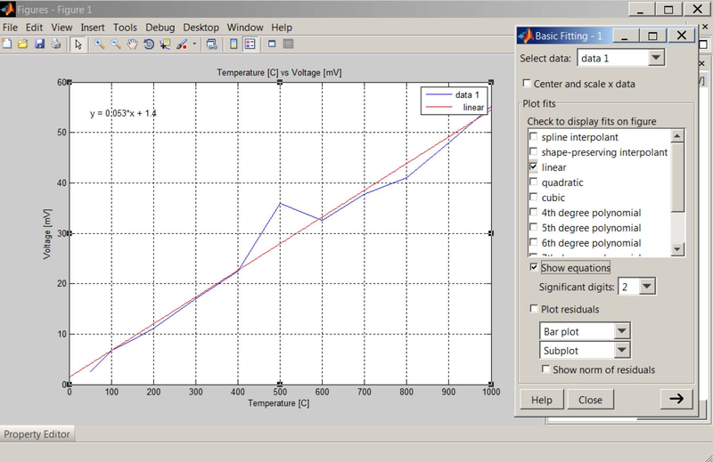
- Plot a graph with Temperature as the independent variable.
- Determine the equation of the relationship using the Basic Fitting tools.
- Estimate the Voltage that corresponds to a Temperature of 650 C and 1150 C.
We will input the variables first:
Temp=[50;100;150;200;/00;400;500;600;700;800;900;1000] Voltage=[2.6;6.7;8.8;11.2;17;22.5;/6;/2.5;/7.7;41;48;55.2]
To plot the graph, type in:
plot(Temp,Voltage)
We can now use the Plot Tools and Basic Fitting settings and determine the equation:
By clicking the right arrow twice at the bottom right corner on the Basic Fitting window, we can evaluate the function at a desired value. See the figure below which illustrates this process for the temperature value 1150 C.
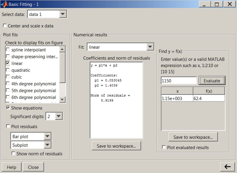
Now let us check our answer with a technique we learned earlier. As displayed on the plot, we have obtained the following equation: y = 0.053x+ 1.4 This equation can be entered as polynomial and evaluated at 650 and 1150 as follows:
    » p=[0.053,1.4]
p =
    0.0530 1.4000
» polyval(p,650)
ans =
    35.8500
» polyval(p,1150)
ans =
    62.3500
- 瀏覽次數:2043
