The efficient frontier with no risk-free asset

Available under Creative Commons-ShareAlike 4.0 International License.

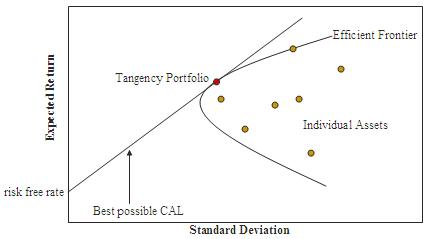
As shown in this graph, every possible combination of the risky assets, without including any holdings of the risk-free asset, can be plotted in risk-expected return space, and the collection of all such possible portfolios defines a region in this space. The left boundary of this region is a hyperbola 1, and the upper edge of this region is the efficient frontier in the absence of a risk-free asset (sometimes called "the Markowitz bullet"). Combinations along this upper edge represent portfolios (including no holdings of the risk-free asset) for which there is lowest risk for a given level of expected return. Equivalently, a portfolio lying on the efficient frontier represents the combination offering the best possible expected return for given risk level.

Figure 9.3

Efficient Frontier. The hyperbola is sometimes referred to as the 'Markowitz Bullet', and is the efficient frontier if no risk-free asset is available. With a risk-free asset, the straight line is the efficient frontier.

Matrices are preferred for calculations of the efficient frontier.

In matrix form, for a given "risk tolerance" $q \in [0,\infty),$ , the efficient frontier is found by minimizing the following expression:

$w^T \Sigma w - q*R^T w$

where

w is a vector of portfolio weights and $\sum_i w_i = 1$ . (The weights can be negative, which means investors can short a security.);

$\Sigma$ is the covariance matrix for the returns on the assets in the portfolio;

$q \ge 0$ is a "risk tolerance" factor, where 0 results in the portfolio with minimal risk and $\infty$ results in the portfolio infinitely far out on the frontier with both expected return and risk unbounded; and

is a vector of expected returns.

$w^T \Sigma w$ is the variance of portfolio return.

R^T w is the expected return on the portfolio.

The above optimization finds the point on the frontier at which the inverse of the slope of the frontier would be q if portfolio return variance instead of standard deviation were plotted horizontally. The frontier in its entirety is parametric on q.

Many software packages, including MATLAB, Microsoft Excel, Mathematica and R, provide optimization routines suitable for the above problem.

An alternative approach to specifying the efficient frontier is to do so parametrically on the expected portfolio return R^T w . This version of the problem requires that we minimize

$w^T \Sigma w$

subject to

$R^T w = \mu$

for parameter $\mu$ . This problem is easily solved using a Lagrange multiplier.

瀏覽次數：10932

您在這裡

The efficient frontier with no risk-free asset