


One of the objectives of the control plane in the network layer is to maintain the routing tables that are used on all routers. As indicated earlier, a routing table is a data structure that contains, for each destination address (or block of addresses) known by the router, the outgoing interface over which the router must forward a packet destined to this address. The routing table may also contain additional information such as the address of the next router on the path towards the destination or an estimation of the cost of this path.
In this section, we discuss the three main techniques that can be used to maintain the routing tables in a network.
Static routing
The simplest solution is to pre-compute all the routing tables of all routers and to install them on each router. Several algorithms can be used to compute these tables.
A simple solution is to use shortest path routing and to minimise the number of intermediate routers to reach each destination. More complex algorithms can take into account the expected load on the links to ensure that congestion does not occur for a given traffic demand. These algorithms must all ensure that :
- all routers are configured with a route to reach each destination
- none of the paths composed with the entries found in the routing tables contain a cycle. Such a cycle would lead to a forwarding loop.
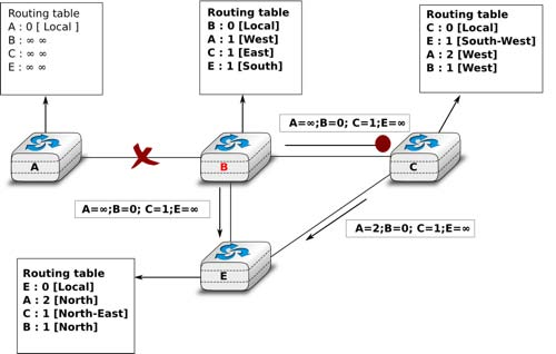
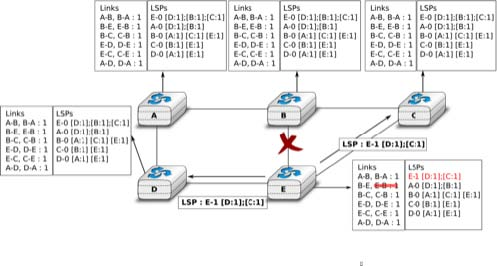
The figure below shows sample routing tables in a five routers network.
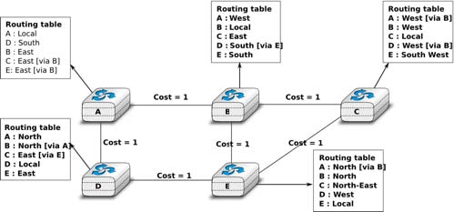
The main drawback of static routing is that it does not adapt to the evolution of the network. When a new router or link is added, all routing tables must be recomputed. Furthermore, when a link or router fails, the routing tables must be updated as well.
Distance vector routing
Distance vector routing is a simple distributed routing protocol. Distance vector routing allows routers to automatically discover the destinations reachable inside the network as well as the shortest path to reach each of these destinations. The shortest path is computed based on metrics or costs that are associated to each link. We use l.cost to represent the metric that has been configured for link l on a router.
Each router maintains a routing table. The routing table R can be modelled as a data structure that stores, for each known destination address d, the following attributes :
- R[d].link is the outgoing link that the router uses to forward packets towards destination d
- R[d].cost is the sum of the metrics of the links that compose the shortest path to reach destination d
- R[d].time is the timestamp of the last distance vector containing destination d
A router that uses distance vector routing regularly sends its distance vector over all its interfaces. The distance vector is a summary of the router’s routing table that indicates the distance towards each known destination. This distance vector can be computed from the routing table by using the pseudo-code below.
Every N seconds: v=Vector() for d in R[]: # add destination d to vector v.add(Pair(d,R[d].cost)) for i in interfaces # send vector v on this interface send(v,interface)
When a router boots, it does not know any destination in the network and its routing table only contains itself. It thus sends to all its neighbours a distance vector that contains only its address at a distance of 0. When a router receives a distance vector on link l, it processes it as follows.
# V : received Vector # l : link over which vector is received def received(V,l):     # received vector from link l
    for din V[]       if not (din R[]) :         # new route         R[d].cost=V[d].cost+l.cost         R[d].link=l         R[d].time=now       else :         # existing route, is the new better ?         if ( ((V[d].cost+l.cost) < R[d].cost) or ( R[d].link == l) ) :             # Better route or change to current route             R[d].cost=V[d].cost+l.cost             R[d].link=l             R[d].time=now
The router iterates over all addresses included in the distance vector. If the distance vector contains an address that the router does not know, it inserts the destination inside its routing table via link l and at a distance which is the sum between the distance indicated in the distance vector and the cost associated to link l. If the destination was already known by the router, it only updates the corresponding entry in its routing table if either :
- the cost of the new route is smaller than the cost of the already known route ( (V[d].cost+l.cost) < R[d].cost)
- the new route was learned over the same link as the current best route towards this destination ( R[d].link == l)
The first condition ensures that the router discovers the shortest path towards each destination. The second condition is used to take into account the changes of routes that may occur after a link failure or a change of the metric associated to a link.
To understand the operation of a distance vector protocol, let us consider the network of five routers shown below.
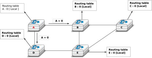
Assume that A is the first to send its distance vector [A=0].
- B and D process the received distance vector and update their routing table with a route towards A.
- D sends its distance vector [D=0,A=1] to A and E. E can now reach A and D.
- C sends its distance vector [C=0] to B and E
- E sends its distance vector [E=0,D=1,A=2,C=2] to D, B and C. B can now reach A, C, D and E
- B sends its distance vector [B=0,A=1,C=1,D=2,E=1] to A, C and E. A, B, C and E can now reach all destinations.
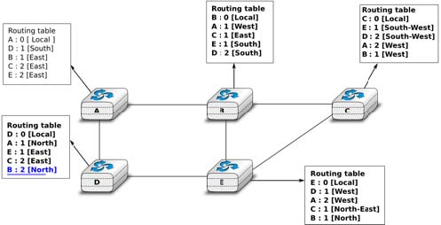
- A sends its distance vector [A=0,B=1,C=2,D=1,E=2] to B and D.
At this point, all routers can reach all other routers in the network thanks to the routing tables shown in the figure below. To deal with link and router failures, routers use the timestamp stored in their routing table. As all routers send their distance vector every N seconds, the timestamp of each route should be regularly refreshed. Thus no route should have a timestamp older than N seconds, unless the route is not reachable anymore. In practice, to cope with the possible loss of a distance vector due to transmission errors, routers check the timestamp of the routes stored in their routing table every N seconds and remove the routes that are older than 3 × N seconds. When a router notices that a route towards a destination has expired, it must first associate an ∞ cost to this route and send its distance vector to its neighbours to inform them. The route can then be removed from the routing table after some time (e.g. 3 × N seconds), to ensure that the neighbouring routers have received the bad news, even if some distance vectors do not reach them due to transmission errors.
Consider the example above and assume that the link between routers A and B fails. Before the failure, A used B to reach destinations B, C and E while B only used the A-B link to reach A. The affected entries timeout on routers A and B and they both send their distance vector.
- A sends its distance vector [A =0,D = ∞,C = ∞,D =1,E = ∞]. D knows that it cannot reach B anymore via A
- D sends its distance vector [D =0,B = ∞,A =1,C =2,E = 1] to A and E. A recovers routes towards C and E via D.
- B sends its distance vector [B =0,A = ∞,C =1,D =2,E = 1] to E and C. D learns that there is no route anymore to reach A via B.
- E sends its distance vector [E =0,A =2,C =1,D =1,B = 1] to D, B and C. D learns a route towards
- C and B learn a route towards A.
At this point, all routers have a routing table allowing them to reach all another routers, except router A, which cannot yet reach router B. A recovers the route towards B once router D sends its updated distance vector [A = 1,B =2,C =2,D =1,E = 1]. This last step is illustrated in figure Routing tables computed by distance vector after a failure, which shows the routing tables on all routers.
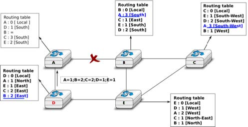
Consider now that the link between D and E fails. The network is now partitioned into two disjoint parts : (A , D) and (B, E, C). The routes towards B, C and E expire first on router D. At this time, router D updates its routing table.
If D sends [D =0,A =1,B = ∞,C = ∞,E = ∞], A learns that B, C and E are unreachable and updates its routing table.
Unfortunately, if the distance vector sent to A is lost or if A sends its own distance vector ( [A =0,D =1,B = 3,C =3,E = 2] ) at the same time as D sends its distance vector, D updates its routing table to use the shorter routes advertised by A towards B, C and E. After some time D sends a new distance vector : [D = 0,A =1,E =3,C =4,B = 4]. A updates its routing table and after some time sends its own distance vector [A =0,D =1,B =5,C =5,E = 4], etc. This problem is known as the count to infinity problem in networking literature. Routers A and D exchange distance vectors with increasing costs until these costs reach ∞. This problem may occur in other scenarios than the one depicted in the above figure. In fact, distance vector routing may suffer from count to infinity problems as soon as there is a cycle in the network. Cycles are necessary to have enough redundancy to deal with link and router failures. To mitigate the impact of counting to infinity, some distance vector protocols consider that 16 = ∞. Unfortunately, this limits the metrics that network operators can use and the diameter of the networks using distance vectors.
This count to infinity problem occurs because router A advertises to router D a route that it has learned via router D. A possible solution to avoid this problem could be to change how a router creates its distance vector. Instead of computing one distance vector and sending it to all its neighbors, a router could create a distance vector that is specific to each neighbour and only contains the routes that have not been learned via this neighbour. This could be implemented by the following pseudocode.
Every N seconds: # one vector for each interface for l in interfaces: v=Vector() for d in R[]: if (R[d].link != i) : v=v+Pair(d,R[d.cost]) send(v) # end for d in R[] #end for l in interfaces
This technique is called split-horizon. With this technique, the count to infinity problem would not have happened in the above scenario, as router A would have advertised [A = 0], since it learned all its other routes via router D. Another variant called split-horizon with poison reverse is also possible. Routers using this variant advertise a cost of ∞ for the destinations that they reach via the router to which they send the distance vector. This can be implemented by using the pseudo-code below.
Every N seconds: for l in interfaces: # one vector for each interface v=Vector() for d in R[]: if (R[d].link != i) : v=v+Pair(d,R[d.cost]) else: v=v+Pair(d,infinity); send(v) # end for d in R[] #end for l in interfaces
Unfortunately, split-horizon, is not sufficient to avoid all count to infinity problems with distance vector routing. Consider the failure of link A-B in the network of four routers below.
After having detected the failure, router A sends its distance vectors :
- [A = ∞,B =0,C = ∞,E = 1] to router C
- [A = ∞,B =0,C =1,E = ∞] to router E
If, unfortunately, the distance vector sent to router C is lost due to a transmission error or because router C is overloaded, a new count to infinity problem can occur. If router C sends its distance vector [A =2,B =1,C = 0,E = ∞] to router E, this router installs a route of distance 3 to reach A via C. Router E sends its distance vectors [A =3,B = ∞,C =1,E = 1] to router B and [A = ∞,B =1,C = ∞,E = 0] to router C. This distance vector allows B to recover a route of distance 4 to reach A.
Link state routing
Link state routing is the second family of routing protocols. While distance vector routers use a distributed algorithm to compute their routing tables, link-state routers exchange messages to allow each router to learn the entire network topology. Based on this learned topology, each router is then able to compute its routing table by using a shortest path computation [Dijkstra1959].
For link-state routing, a network is modelled as a directed weighted graph. Each router is a node, and the links between routers are the edges in the graph. A positive weight is associated to each directed edge and routers use the shortest path to reach each destination. In practice, different types of weight can be associated to each directed edge :
- unit weight. If all links have a unit weight, shortest path routing prefers the paths with the least number of intermediate routers.
- weight proportional to the propagation delay on the link. If all link weights are configured this way, shortest path routing uses the paths with the smallest propagation delay.
- where C is a constant larger than the highest link bandwidth in the network. If all link weights are configured this way, shortest path routing prefers higher bandwidth paths over lower bandwidth paths
Usually, the same weight is associated to the two directed edges that correspond to a physical link (i.e. R1 → R2 and R2 → R1). However, nothing in the link state protocols requires this. For example, if the weight is set in function of the link bandwidth, then an asymmetric ADSL link could have a different weight for the upstream and downstream directions. Other variants are possible. Some networks use optimisation algorithms to find the best set of weights to minimize congestion inside the network for a given traffic demand [FRT2002].
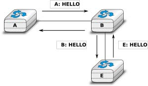
When a link-state router boots, it first needs to discover to which routers it is directly connected. For this, each router sends a HELLO message every N seconds on all of its interfaces. This message contains the router’s address. Each router has a unique address. As its neighbouring routers also send HELLO messages, the router automatically discovers to which neighbours it is connected. These HELLO messages are only sent to neighbours who are directly connected to a router, and a router never forwards the HELLO messages that they receive. HELLO messages are also used to detect link and router failures. A link is considered to have failed if no HELLO message has been received from the neighbouring router for a period of k × N seconds.
Once a router has discovered its neighbours, it must reliably distribute its local links to all routers in the network to allow them to compute their local view of the network topology. For this, each router builds a link-state packet (LSP) containing the following information :
- LSP.Router : identification (address) of the sender of the LSP
- LSP.age : age or remaining lifetime of the LSP
- LSP.seq : sequence number of the LSP
- LSP.Links[] : links advertised in the LSP. Each directed link is represented with the following information : -LSP.Links[i].Id : identification of the neighbour -LSP.Links[i].cost : cost of the link
These LSPs must be reliably distributed inside the network without using the router’s routing table since these tables can only be computed once the LSPs have been received. The Flooding algorithm is used to efficiently distribute the LSPs of all routers. Each router that implements flooding maintains a link state database (LSDB) containing the most recent LSP sent by each router. When a router receives an LSP, it first verifies whether this LSP is already stored inside its LSDB. If so, the router has already distributed the LSP earlier and it does not need to forward it. Otherwise, the router forwards the LSP on all links except the link over which the LSP was received. Reliable flooding can be implemented by using the following pseudo-code.
# links is the set of all links on the router # Router R’s LSP arrival on link l if newer(LSP, LSDB(LSP.Router)) : LSDB.add(LSP) for i in links : if i!=l : send(LSP,i) else: # LSP has already been flooded
In this pseudo-code, LSDB(r) returns the most recent LSP originating from router r that is stored in the LSDB. newer(lsp1,lsp2) returns true if lsp1 is more recent than lsp2. See the note below for a discussion on how newer can be implemented.
A router that implements flooding must be able to detect whether a received LSP is newer than the stored LSP. This requires a comparison between the sequence number of the received LSP and the sequence number of the LSP stored in the link state database. The ARPANET routing protocol [MRR1979] used a 6 bits sequence number and implemented the comparison as follows RFC 789
def newer( lsp1, lsp2 ): return ( ( ( lsp1.seq > lsp2.seq) and ( (lsp1.seq-lsp2.seq)<=32) ) or ( ( lsp1.seq < lsp2.seq) and ( (lsp2.seq-lsp1.seq)> 32) ) )This comparison takes into account the modulo 2 arithmetic used to increment the sequence numbers. Intuitively, the comparison divides the circle of all sequence numbers into two halves. Usually, the sequence number of the received LSP is equal to the sequence number of the stored LSP incremented by one, but sometimes the sequence numbers of two successive LSPs may differ, e.g. if one router has been disconnected from the network for some time. The comparison above worked well until October 27, 1980. On this day, the ARPANET crashed completely. The crash was complex and involved several routers. At one point, LSP 40 and LSP 44 from one of the routers were stored in the LSDB of some routers in the ARPANET. As LSP 44 was the newest, it should have replaced by LSP 40 on all routers. Unfortunately, one of the ARPANET routers suffered from a memory problem and sequence number 40 (101000 in binary) was replaced by 8 (001000 in binary) in the buggy router and flooded. Three LSPs were present in the network and 44 was newer than 40 which is newer than 8, but unfortunately 8 was considered to be newer than 44... All routers started to exchange these three link state packets for ever and the only solution to recover from this problem was to shutdown the entire network RFC 789.
Current link state routing protocols usually use 32 bits sequence numbers and include a special mechanism in the unlikely case that a sequence number reaches the maximum value (using a 32
bits sequence number space takes 136 years if a link state packet is generated every second).
To deal with the memory corruption problem, link state packets contain a checksum. This checksum is computed by the router that generates the LSP. Each router must verify the checksum when it
receives or floods an LSP. Furthermore, each router must periodically verify the checksums of the LSPs stored in its LSDB.
Flooding is illustrated in the figure below. By exchanging HELLO messages, each router learns its direct neighbours. For example, router E learns that it is directly connected to
routers D, B and C. Its first LSP has sequence number 0 and contains the directed links E->D, E->B and E->C. Router
E sends its LSP on all its links and routers D, B and C insert the LSP in their LSDB and forward it over their other links.
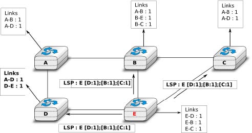
Flooding allows LSPs to be distributed to all routers inside the network without relying on routing tables. In the example above, the LSP sent by router E is likely to be sent twice on some links in the network. For example, routers B and C receive E‘s LSP at almost the same time and forward it over the B-C link. To avoid sending the same LSP twice on each link, a possible solution is to slightly change the pseudo-code above so that a router waits for some random time before forwarding a LSP on each link. The drawback of this solution is that the delay to flood an LSP to all routers in the network increases. In practice, routers immediately flood the LSPs that contain new information (e.g. addition or removal of a link) and delay the flooding of refresh LSPs (i.e. LSPs that contain exactly the same information as the previous LSP originating from this router) [FFEB2005].
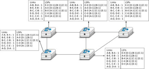
To ensure that all routers receive all LSPs, even when there are transmissions errors, link state routing protocols use reliable flooding. With reliable flooding, routers use acknowledgements and if necessary retransmissions to ensure that all link state packets are successfully transferred to all neighbouring routers. Thanks to reliable flooding, all routers store in their LSDB the most recent LSP sent by each router in the network. By combining the received LSPs with its own LSP, each router can compute the entire network topology.
As link state packets are flooded regularly, routers are able to measure the quality (e.g. delay or load) of their links and adjust the metric of each link according to its current quality. Such dynamic adjustments were included in the ARPANET routing protocol [MRR1979] . However, experience showed that it was difficult to tune the dynamic adjustments and ensure that no forwarding loops occur in the network [KZ1989]. Today’s link state routing protocols use metrics that are manually configured on the routers and are only changed by the network operators or network management tools [FRT2002].
When a link fails, the two routers attached to the link detect the failure by the lack of HELLO messages received in the last k × N seconds. Once a router has detected a local link failure, it generates and floods a new LSP that no longer contains the failed link and the new LSP replaces the previous LSP in the network. As the two routers attached to a link do not detect this failure exactly at the same time, some links may be announced in only one direction. This is illustrated in the figure below. Router E has detected the failures of link E-B and flooded a new LSP, but router B has not yet detected the failure.
When a link is reported in the LSP of only one of the attached routers, routers consider the link as having failed and they remove it from the directed graph that they compute from their LSDB. This is called the two-way connectivity check. This check allows link failures to be flooded quickly as a single LSP is sufficient to announce such bad news. However, when a link comes up, it can only be used once the two attached routers have sent their LSPs. The two-way connectivity check also allows for dealing with router failures. When a router fails, all its links fail by definition. Unfortunately, it does not, of course, send a new LSP to announce its failure. The two-way connectivity check ensures that the failed router is removed from the graph.
When a router has failed, its LSP must be removed from the LSDB of all routers 1. This can be done by using the age field that is included in each LSP. The age field is used to bound the maximum lifetime of a link state packet in the network. When a router generates a LSP, it sets its lifetime (usually measured in seconds) in the age field. All routers regularly decrement the age of the LSPs in their LSDB and a LSP is discarded once its age reaches 0. Thanks to the age field, the LSP from a failed router does not remain in the LSDBs forever.
To compute its routing table, each router computes the spanning tree rooted at itself by using Dijkstra’s shortest path algorithm [Dijkstra1959]. The routing table can be derived automatically from the spanning as shown in the figure below.
- 3646 reads
