


Probabilities are calculated by using technology. There are instructions in the chapter for the TI-83+ and TI-84 calculators.
Example 3.4
If the area to the left is 0.0228, then the area to the right is 1 − 0.0228 = 0.9772.
Example 3.5
The final exam scores in a statistics class were normally distributed with a mean of 63 and a standard deviation of 5.
Please see Problem 1-4.
Problem 1
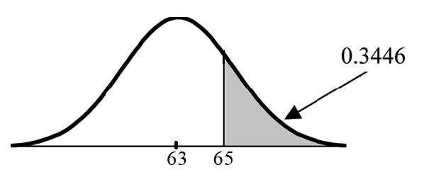
Find the probability that a randomly selected student scored more than 65 on the exam.
Solution
Let X = a score on the final exam. X∼N (63, 5), where µ = 63 and σ = 5 Draw a graph.
Then, find P (x> 65).
P (x> 65) = 0.3446 (calculator or computer)
 The probability that one student scores more than 65 is
0.3446. Using the TI-83+ or the TI-84 calculators, the calculation is as follows. Go into 2nd DISTR. After pressing 2nd DISTR, press 2:normalcdf. The syntax for the instructions are shown
below. normalcdf(lower value, upper value, mean, standard deviation) For this problem: normal cdf(65,1E99,63,5) = 0.3446. You get 1E99 ( 1099) by pressing 1, the EE key (a 2nd key) and then 99. Or, you can enter 10-99 instead. The number 1099 is way out in the right tail of the normal curve. We are calculating the area between 65 and
1099 . In some instances, the lower number of the area might be -1E99 ( −1099). The number −1099 is way out in the left tail of the normal curve.
The probability that one student scores more than 65 is
0.3446. Using the TI-83+ or the TI-84 calculators, the calculation is as follows. Go into 2nd DISTR. After pressing 2nd DISTR, press 2:normalcdf. The syntax for the instructions are shown
below. normalcdf(lower value, upper value, mean, standard deviation) For this problem: normal cdf(65,1E99,63,5) = 0.3446. You get 1E99 ( 1099) by pressing 1, the EE key (a 2nd key) and then 99. Or, you can enter 10-99 instead. The number 1099 is way out in the right tail of the normal curve. We are calculating the area between 65 and
1099 . In some instances, the lower number of the area might be -1E99 ( −1099). The number −1099 is way out in the left tail of the normal curve.
Area to the left is 0.6554. P (x> 65) = P (z> 0.4) = 1 − 0.6554 = 0.3446
Problem 2
Find the probability that a randomly selected student scored less than 85.
Solution
Draw a graph. Then find P (x< 85). Shade the graph. P (x< 85) = 1 (calculator or computer) The probability that one student scores less than 85 is approximately 1 (or 100%). The
TI-instructions and answer are as follows: normalcdf(0,85,63,5) = 1 (rounds to 1)
Problem 3
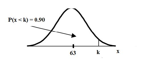
Find the 90th percentile (that is, find the score k that has 90 % of the scores below k and 10% of the scores above k).
Solution
Find the 90th percentile. For each problem or part of a problem, draw a new graph. Draw the x-axis. Shade the area that corresponds to the 90th percentile.
Let k = the 90th percentile. k is located on the x-axis. P (x<k) is the area to the left of k. The 90th percentile k separates the exam scores into those that
are the same or lower than k and those that are the same or higher. Ninety percent of the test scores are the same or lower than k and 10% are the same or higher. k is often called a
critical value.
k = 69.4 (calculator or computer)
The 90th percentile is 69.4. This means that 90% of the test scores fall at or below 69.4 and 10% fall at or above. For the TI-83+ or TI-84 calculators, use invNorm in 2nd DISTR. invNorm(area
to the left, mean, standard deviation) For this problem, invNorm(0.90,63,5) = 69.4
Problem 4
Find the 70th percentile (that is, find the score k such that 70% of scores are below k and 30% of the scores are above k).
Solution
Find the 70th percentile.
Draw a new graph and label it appropriately. k = 65.6
The 70th percentile is 65.6. This means that 70% of the test scores fall at or below 65.5 and 30% fall at or above.
invNorm(0.70,63,5) = 65.6
Example 3.6
A computer is used for office work at home, research, communication, personal finances, education, entertainment, social networking and a myriad of other things. Suppose that the average
number of hours a household personal computer is used for entertainment is 2 hours per day. Assume the times for entertainment are normally distributed and the standard deviation for the
times is half an hour.
Please see problem 1-2.
Problem 1
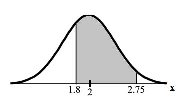
Find the probability that a household personal computer is used between 1.8 and 2.75 hours per day.
Solution
Let X = the amount of time (in hours) a household personal computer is used for entertainment. x∼N (2, 0.5) where µ = 2 and σ = 0.5.
Find P (1.8 <x< 2.75).
The probability for which you are looking is the area between x = 1.8 and x = 2.75. P (1.8 <x< 2.75) = 0.5886
normalcdf(1.8,2.75,2,0.5) = 0.5886
The probability that a household personal computer is used between 1.8 and 2.75 hours per day for entertainment is 0.5886.
Problem 2
Find the maximum number of hours per day that the bottom quartile of households use a personal computer for entertainment.
Solution
To find the maximum number of hours per day that the bottom quartile of households uses a personal computer for entertainment,find the 25th
percentile, k, where P (x<k) = 0.25.
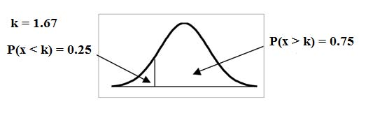 invNorm(0.25,2,.5) = 1.66
The maximum number of hours per day that the bottom quartile of households uses a personal computer for entertainment is 1.66 hours.
- 8498 reads
