Law of Large Numbers
The Law of Large Numbers says that if you take samples of larger and larger size from any population, then the mean  of the sample tends to get closer and closer to µ. From the Central Limit Theorem, we know
that as n gets larger and larger, the sample means follow a normal distribution. The larger n gets, the smaller the standard deviation gets. (Remember that the standard deviation
for
  is
is  .) This means that the sample mean
  must be close to the population mean µ. We can say that µ is the value that the sample
means approach as n gets larger. The Central Limit Theorem illustrates the Law of Large Numbers.
Central Limit Theorem for the Mean and Sum Examples
Example 3.9
A study involving stress is done on a college campus among the students. The stress scores follow a uniform distribution with the lowest stress score equal to 1 and the highest equal to 5. Using a sample of 75 students, find:
- The probability that the mean stress score for the 75 students is less than 2.
- The 90th percentile for the mean stress score for the 75 students.
- The probability that the total of the 75 stress scores is less than 200.
- The 90th percentile for the total stress score for the 75 students.
Let X = one stress score.
Problems 1 and 2 ask you to find a probability or a percentile for a mean. Problems 3 and 4 ask you to find a probability or a percentile for a total or sum.
The sample size, n, is equal to 75.
Since the individual stress scores follow a uniform distribution, X ∼ U (1, 5) where a = 1 and b = 5 (See Continuous Random Variables for the uniform).
For problems 1. and 2., let
 = the mean stress score for the 75
students. Then,
  where n =
75.
See Problem 1-4.
Problem 1
Find  . Draw the graph.
Solution
 The probability that the mean stress score is
less than 2 is about 0.
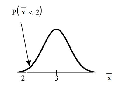
 REMINDER: The smallest stress score
is 1. Therefore, the smallest mean for 75 stress scores is 1.
Problem 2
Find the 90th percentile for the mean of 75 stress scores. Draw a graph.
Solution
Let k = the 90th percentile.
Find k where 
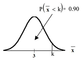 The 90th percentile for the mean of 75 scores is about
3.2. This tells us that 90% of all the means of 75 stress scores are at most 3.2 and 10% are at least 3.2.
  For problems c and d, let ΣX = the sum of the 75 stress scores. Then,
![\sum X\sim N[(75)\cdot(3),\sqrt{75}\cdot 1.15]](/system/files/resource/9/9418/9462/media/eqn-img_97.gif)
Problem 3
Find P (Σx < 200). Draw the graph.
Solution
The mean of the sum of 75 stress scores is 75 · 3 = 225
The standard deviation of the sum of 75 stress scores is
P (Σx < 200) = 0 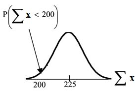 The probability that the total of
75 scores is less than 200 is about 0.
  REMINDER: The smallest total of 75 stress scores is 75 since the smallest single score is 1.
Problem 4
Find the 90th percentile for the total of 75 stress scores. Draw a graph.
Solution
Let k = the 90th percentile.
Find k where P (Σx <k) = 0.90.
k = 237.8 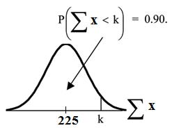 The 90th percentile for the sum of 75 scores
is about 237.8. This tells us that 90% of all the sums of 75 scores are no more than 237.8 and 10% are no less than 237.8.
Example 3.10
Suppose that a market research analyst for a cell phone company conducts a study of their customers who exceed the time allowance included on their basic cell phone contract; the analyst
finds that for those people who exceed the time included in their basic contract, the excess time used follows an exponential distribution with a mean of 22
minutes.
Consider a random sample of 80 customers who exceed the time allowance included in their basic cell phone contract.
Let X = the excess time used by one INDIVIDUAL cell phone customer who exceeds his contracted time allowance.  From Chapter 5, we know that µ = 22 and σ = 22.
Let  = the mean excess time used by a sample of n = 80
customers who exceed their contracted time allowance.
  by the CLT for Sample Means.
See Problems 5-6.
Problem 5
Using the CLT to find Probability:
- Find the probability that the mean excess time used by the 80 customers in the sample is longer than 20 minutes. This is asking us to find
Draw the graph.
- Suppose that one customer who exceeds the time limit for his cell phone contract is randomly selected. Find the probability that this individual customer's excess time is longer than 20 minutes. This is asking us to find P (x > 20)
- Explain why the probabilities in (a) and (b) are different.
Solution
Part a.
Find: 
 using
using The
probability is 0.7919 that the mean excess time used is more than 20 minutes, for a sample of 80 customers who exceed their contracted time allowance.
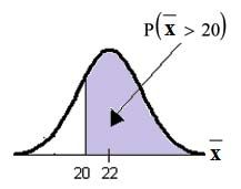 REMINDER: 1E99 = 1099 and−1E99 = −1099 . Press the EE key for E. Or
just use 10^99 instead of 1E99.
Part b.
Find P(x>20) . Remember to use the exponential distribution for an individual: X∼Exp(1/22).
Part c. Explain why the probabilities in (a) and (b) are different.
The probabilities are not equal because we use different distributions to calculate the probability for individuals and for means.
When asked to find the probability of an individual value, use the stated distribution of its random variable; do not use the CLT. Use the CLT with the normal distribution when you are being
asked to find the probability for an mean.
Problem 6
Using the CLT to find Percentiles:
Find the 95th percentile for the sample mean excess time for samples of 80 customers who exceed their basic contract time allowances. Draw
a graph.
Solution
Let k = the 95th percentile. Find k where 
k = 26.0 using
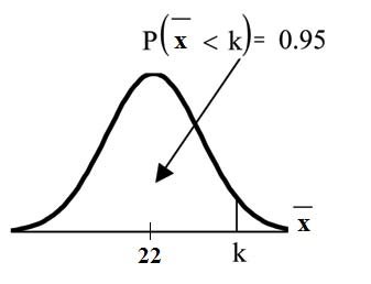 The 95th percentile for the sample mean excess time used is about 26.0 minutes for random samples of 80 customers who exceed their contractual allowed time. 95% of such samples would have means under 26
minutes; only 5% of such samples would have means above 26 minutes.
- there are a certain number n of independent trials
- the outcomes of any trial are success or failure
- each trial has the same probability of a success p
Recall that if X is the binomial random variable, then X∼B (n, p). The shape of the binomial distribution needs to be similar to the shape of the normal distribution. To ensure this, the
quantities np and nq must both be greater than five (np > 5 and nq > 5; the approximation is better if they are both greater than or equal to 10). Then the binomial can be approximated
by the normal distribution with mean µ = np and standard deviation  . Remember that q = 1 − p. In order to get the best approximation, add 0.5 to x or subtract 0.5 from x (use x + 0.5 or x − 0.5).
The number 0.5 is called the continuity correction factor.
Example 3.11
Suppose in a local Kindergarten through 12th grade (K - 12) school district, 53 percent of the population favor a charter school for grades K - 5. A simple random sample of 300 is surveyed.
- Find the probability that at least 150 favor a charter school.
- Find the probability that at most 160 favor a charter school.
- Find the probability that more than 155 favor a charter school.
- Find the probability that less than 147 favor a charter school.
- Find the probability that exactly 175 favor a charter school.
Let X = the number that favor a charter school for grades K - 5. X∼B (n, p) where n = 300 and p = 0.53. Since np > 5 and nq > 5, use the normal approximation to the binomial. The
formulas for the mean and standard deviation are µ = np and  . The mean is 159 and the standard deviation is 8.6447. The random variable for the normal distribution is Y
.Y ∼ N (159, 8.6447). See The Normal Distribution for help
with calculator instructions.
For Problem 1., you include 150 so P (x ≥ 150) has normal approximation P (Y ≥ 149.5) = 0.8641.  For Problem 2., you include 160 so P (x ≤ 160) has normal approximation
P (Y ≤ 160.5) = 0.5689.
  For Problem 3.,
you exclude 155 so P (x > 155) has normal approximation P (y > 155.5) = 0.6572.
  For Problem 4., you exclude 147 so P (x < 147) has normal
approximation P (Y < 146.5) = 0.0741.
  For Problem 5., P (x = 175) has normal approximation P (174.5 < y < 175.5) = 0.0083.
Because of calculators and computer software that easily let you calculate binomial probabilities for large values of n, it is not necessary to use the the
Normal Approximation to the Binomial provided you have access to these technology tools. Most school labs have Microsoft Excel, an example of computer software that calculates binomial
probabilities. Many students have access to the TI-83 or 84 series calculators and they easily calculate probabilities for the binomial. In an Internet browser, if you type in "binomial
probability distribution calculation," you can find at least one online calculator for the binomial.
For Example 3, the probabilities are calculated using the binomial (n = 300 and p = 0.53) below. Compare the binomial and normal distribution answers. See
Discrete Random Variables for help with calculator instructions for the binomial.
P (x ≥ 150): 1 - binomialcdf (300, 0.53, 149) = 0.8641
P (x ≤ 160): binomialcdf (300, 0.53, 160) = 0.5684
P (x > 155): 1 - binomialcdf (300, 0.53, 155) = 0.6576
P (x < 147): binomialcdf (300, 0.53, 146) = 0.0742
P (x = 175): (You use the binomial pdf.) binomialpdf (175, 0.53, 146) = 0.0083
**Contributions made to Example 2 by Roberta Bloom
- 24558 reads


