


Data may come from a population or from a sample. Small letters like x or y generally are used to represent data values. Most data can be put into the following categories:
- Qualitative
- Quantitative
Qualitative data are the result of categorizing or describing attributes of a population. Hair color, blood type, ethnic group, the car a person drives, and the street a person lives on are examples of qualitative data. Qualitative data are generally described by words or letters. For instance, hair color might be black, dark brown, light brown, blonde, gray, or red. Blood type might be AB+, O-, or B+. Researchers often prefer to use quantitative data over qualitative data because it lends itself more easily to mathematical analysis. For example, it does not make sense to find an average hair color or blood type.
Quantitative data are always numbers. Quantitative data are the result of counting or measuring attributes of a population. Amount of money, pulse rate, weight, number of people living in your town, and the number of students who take statistics are examples of quantitative data. Quantitative data may be either discrete or continuous.
All data that are the result of counting are called quantitative discrete data. These data take on only certain numerical values. If you count the number of phone calls you receive for each day of the week, you might get 0, 1, 2, 3, etc.
All data that are the result of measuring are quantitative continuous data assuming that we can measure accurately. Measuring angles in radians might result in the
numbers  , etc.
If you and your friends carry backpacks with books in them to school, the numbers of books in the backpacks are discrete data and the weights of the backpacks are continuous data.
, etc.
If you and your friends carry backpacks with books in them to school, the numbers of books in the backpacks are discrete data and the weights of the backpacks are continuous data.
Example 1.2: Data Sample of Quantitative Discrete Data
The data are the number of books students carry in their backpacks. You sample five students. Two students carry 3 books, one student carries 4 books, one student carries 2 books, and one student carries 1 book. The numbers of books (3, 4, 2, and 1) are the quantitative discrete data.
Example 1.3: Data Sample of Quantitative Continuous Data
The data are the weights of the backpacks with the books in it. You sample the same five students. The weights (in pounds) of their backpacks are 6.2, 7, 6.8, 9.1, 4.3. Notice that backpacks carrying three books can have different weights. Weights are quantitative continuous data because weights are measured.
Example 1.4: Data Sample of Qualitative Data
The data are the colors of backpacks. Again, you sample the same five students. One student has a red backpack, two students have black backpacks, one student has a green backpack, and one student has a gray backpack. The colors red, black, black, green, and gray are qualitative data.
Example 1.5
Work collaboratively to determine the correct data type (quantitative or qualitative). Indicate whether quantitative data are continuous or discrete. Hint: Data that are discrete often start with the words "the number of."
- The number of pairs of shoes you own.
- The type of car you drive.
- Where you go on vacation.
- The distance it is from your home to the nearest grocery store.
- The number of classes you take per school year.
- The tuition for your classes
- The type of calculator you use.
- Movie ratings.
- Political party preferences.
- Weight of sumo wrestlers.
- Amount of money won playing poker.
- Number of correct answers on a quiz.
- Peoples' attitudes toward the government.
- IQ scores. (This may cause some discussion.)
Qualitative Data Discussion
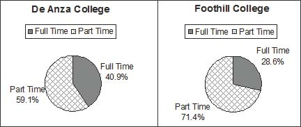
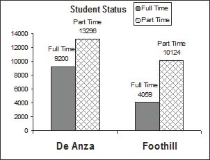
Below are tables of part-time vs full-time students at De Anza College in Cupertino, CA and Foothill College in Los Altos, CA for the Spring 2010 quarter. The tables display counts (frequencies) and percentages or proportions (relative frequencies). The percent columns make comparing the same categories in the colleges easier. Displaying percentages along with the numbers is often helpful, but it is particularly important when comparing sets of data that do not have the same totals, such as the total enrollments for both colleges in this example. Notice how much larger the percentage for part-time students at Foothill College is compared to De Anza College.
|
Number |
Percent |
|
|---|---|---|
|
Full-time |
9,200 |
40.9% |
|
Part-time |
13,296 |
59.1% |
|
Total |
22,496 |
100% |
|
Number |
Percent |
|
|---|---|---|
|
Full-time |
4,059 |
28.6% |
|
Part-time |
10,124 |
71.4% |
|
Total |
14,183 |
100% |
Tables are a good way of organizing and displaying data. But graphs can be even more helpful in understanding the data. There are no strict rules concerning what graphs to use. Below are pie charts and bar graphs, two graphs that are used to display qualitative data.
In a pie chart, categories of data are represented by wedges in the circle and are proportional in size to the percent of individuals in each category.
In a bar graph, the length of the bar for each category is proportional to the number or percent of individuals in each category. Bars may be vertical or horizontal.
A Pareto chart consists of bars that are sorted into order by category size (largest to smallest).
Look at the graphs and determine which graph (pie or bar) you think displays the comparisons better. This is a matter of preference.
It is a good idea to look at a variety of graphs to see which is the most helpful in displaying the data. We might make different choices of what we think is the "best" graph depending on the data and the context. Our choice also depends on what we are using the data for.
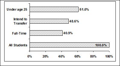
Percentages That Add to More (or Less) Than 100%
Sometimes percentages add up to be more than 100% (or less than 100%). In the graph, the percentages add to more than 100% because students can be in more than one category. A bar graph is appropriate to compare the relative size of the categories. A pie chart cannot be used. It also could not be used if the percentages added to less than 100%.
|
Characteristic/Category |
Percent |
|---|---|
|
Full-time Students |
40.9% |
|
Students who intend to transfer to a 4-year educational institution |
48.6% |
|
Students under age 25 |
61.0% |
|
TOTAL |
150.5% |
Omitting Categories/Missing Data
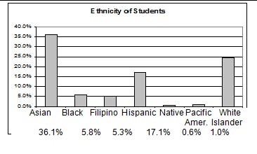
The table displays Ethnicity of Students but is missing the "Other/Unknown" category. This category contains people who did not feel they fit into any of the ethnicity categories or declined to respond. Notice that the frequencies do not add up to the total number of students. Create a bar graph and not a pie chart.
|
Frequency |
Percent |
|
|---|---|---|
|
Asian |
8,794 |
36.1% |
|
Black |
1,412 |
5.8% |
|
Filipino |
1,298 |
5.3% |
|
Hispanic |
4,180 |
17.1% |
|
Native American |
146 |
0.6% |
|
Pacifc Islander |
236 |
1.0% |
|
White |
5,978 |
24.5% |
|
TOTAL |
22,044 out of 24,382 |
90.4% out of 100% |
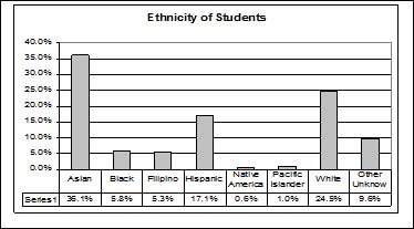
The following graph is the same as the previous graph but the "Other/Unknown" percent (9.6%) has been added back in. The "Other/Unknown" category is large compared to some of the other categories (Native American, 0.6%, Pacifc Islander 1.0% particularly). This is important to know when we think about what the data are telling us.
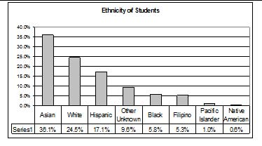
This particular bar graph can be hard to understand visually. The graph below it is a Pareto chart. The Pareto chart has the bars sorted from largest to smallest and is easier to read and interpret.
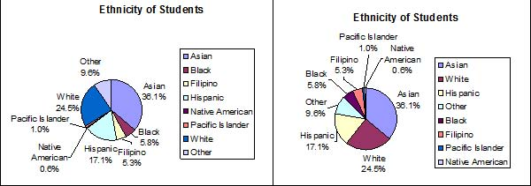
Pie Charts: No Missing Data
The following pie charts have the "Other/Unknown" category added back in (since the percentages must add to 100%). The chart on the right is organized having the wedges by size and makes for a more visually informative graph than the unsorted, alphabetical graph on the left.
- 5398 reads
