


The correlation coefficient, r, tells us about the strength of the linear relationship between x and y. However, the reliability of the linear model also depends on how many observed data points are in the sample. We need to look at both the value of the correlation coefficient r and the sample size n, together.
We perform a hypothesis test of the "significance of the correlation coefficient" to decide whether the linear relationship in the sample data is strong enough to use to model the relationship in the population.
The sample data is used to computer r, the correlation coefficient for the sample. If we had data for the entire population, we could find the population correlation coefficient. But because we only have sample data, we can not calculate the population correlation coefficient. The sample correlation coefficient, r, is our estimate of the unknown population correlation coefficient.
The symbol for the population correlation coefficient is ρ, the Greek letter "rho".
ρ = population correlation coefficient (unknown)
r = sample correlation coefficient (known; calculated from sample data)
The hypothesis test lets us decide whether the value of the population correlation coefficient ρ is "close to 0" or "significantly different from 0". We decide this based on the sample correlation coefficient r and the sample size n.
If the test concludes that the correlation coefficient is significantly different from 0, we say that the correlation coefficient is "significant".
- Conclusion: "There is sufficient evidence to conclude that there is a significant linear relationship between x and y because the correlation coefficient is significantly different from 0."
- What the conclusion means: There is a significant linear relationship between x and y. We can use the regression line to model the linear relationship between x and y in the population.
If the test concludes that the correlation coefficient is not significantly different from 0 (it is close to 0), we say that correlation coefficient is "not significant".
- Conclusion: "There is insufficient evidence to conclude that there is a significant linear relationship between x and y because the correlation coefficient is not significantly different from 0."
- What the conclusion means: There is not a significant linear relationship between x and y. Therefore we can NOT use the regression line to model a linear relationship between x and y in the population.
- If r is significant and the scatter plot shows a linear trend, the line can be used to predict the value of y for values of x that are within the domain of observed x values.
- If r is not significant OR if the scatter plot does not show a linear trend, the line should not be used for prediction.
- If r is significant and if the scatter plot shows a linear trend, the line may NOT be appropriate or reliable for prediction OUTSIDE the domain of observed x values in the data.
PERFORMING THE HYPOTHESIS TEST
SETTING UP THE HYPOTHESES:
-
Null Hypothesis:

-
Alternate Hypothesis:

What the hypotheses mean in words:
- Null Hypothesis Ho: The population correlation coefficient IS NOT significantly different from 0. There IS NOT a significant linear relationship(correlation) between x and y in the population.
- Alternate Hypothesis Ha: The population correlation coefficient IS significantly DIFFERENT FROM 0. There IS A SIGNIFICANT LINEAR RELATIONSHIP (correlation) between x and y in the population.
DRAWING A CONCLUSION:
There are two methods to make the decision. Both methods are equivalent and give the same result.
Method 1: Using the p-value
Method 2: Using a table of critical values
In this chapter of this textbook, we will always use a significance level of 5%, α = 0.05
METHOD 1: Using a p-value to make a decision
On the LinRegTTEST input screen, on the line prompt for β or ρ, highlight " 0"
0"
The output screen shows the p-value on the line that reads "p = ".
(Most computer statistical software can calculate the p-value.)
If the p-value is less than the significance level (α = 0.05):
- Decision: REJECT the null hypothesis.
- Conclusion: "There is sufficient evidence to conclude that there is a significant linear relationship between x and y because the correlation coefficient is significantly different from 0."
If the p-value is NOT less than the significance level (α = 0.05):
- Decision: DO NOT REJECT the null hypothesis.
- Conclusion: "There is insufficient evidence to conclude that there is a significant linear relationship between x and y because the correlation coefficient is NOT significantly different from 0."
Calculation Notes:
You will use technology to calculate the p-value. The following describe the calculations to compute the test statistics and the p-value:
The p-value is calculated using a t-distribution with n − 2 degrees of freedom.
The formula for the test statistic is  . The value of the test statistic, t, is shown in the computer or calculator output along with the p-value. The test
statistic t has the same sign as the correlation coefficient r.
. The value of the test statistic, t, is shown in the computer or calculator output along with the p-value. The test
statistic t has the same sign as the correlation coefficient r.
The p-value is the combined area in both tails.
An alternative way to calculate the p-value (p) given by LinRegTTest is the command 2*tcdf(abs(t),10^99, n-2) in 2nd DISTR.
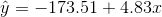
THIRD EXAM vs FINAL EXAM EXAMPLE: p value method
- Consider the third exam/final exam example.
- The line of best fit is:
 with r =0.6631 and
there are n = 11 data points.
with r =0.6631 and
there are n = 11 data points.
- Can the regression line be used for prediction? Given a third exam score (x value), can we use the line to predict the final exam score (predicted y value)?

The p-value is 0.026 (from LinRegTTest on your calculator or from computer software)
The p-value, 0.026, is less than the signifcance level of α = 0.05
Decision: Reject the Null Hypothesis Ho
Conclusion: There is sufcient evidence to conclude that there is a significant linear relationship between x and y because the correlation coefficient is significantly
different from 0.
Because r is significant and the scatter plot shows a linear trend, the regression line can be used to predict final exam scores.
METHOD 2: Using a table of Critical Values to make a decision
The 95% Critical Values of the Sample Correlation Coefficient Table at the end of this chapter (before the Summary) may be used to give you a good idea of whether the computed value of r is significant or not. Compare r to the appropriate critical value in the table. If r is not between the positive and negative critical values, then the correlation coefficient is significant. If r is significant, then you may want to use the line for prediction.
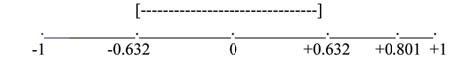
Example 6.7
Suppose you computed r =0.801 using n = 10 data points. df = n − 2 = 10 − 2= 8. The critical values associated with df = 8 are -0.632 and + 0.632. If r<
negative critical value or r> positive critical value, then r is significant. Since r = 0.801 and 0.801 > 0.632, r is significant and the line may be
used for prediction. If you view this example on a number line, it will help you.
Example 6.8
Suppose you computed r = −0.624 with 14 data points. df = 14 − 2 = 12. The critical values are -0.532 and 0.532. Since −0.624<−0.532, r is significant and the line may be
used for prediction

Example 6.9
Suppose you computed r = 0.776 and n = 6. df = 6 − 2= 4. The critical values are -0.811 and 0.811. Since −0.811 < 0.776 < 0.811, r is not significant and the line should not be used for prediction.

THIRD EXAM vs FINAL EXAM EXAMPLE: critical value method
- Consider the third exam final exam example.
- The line of best fit is:
 with r =
0.6631 and there are n = 11 data points.
with r =
0.6631 and there are n = 11 data points.
- Can the regression line be used for prediction? Given a third exam score (x value), can we use the line to predict the final exam score (predicted y value)?

Use the "95% Critical Value" table for r with df = n − 2 = 11 − 2 = 9
The critical values are -0.602 and +0.602
Since 0.6631 > 0.602, r is significant.
Decision: Reject Ho:
Conclusion: There is sufficient evidence to conclude that there is a significant linear relationship between x and y because the correlation coefficient is significantly different from 0.
Because r is significant and the scatter plot shows a linear trend, the regression line can be used to predict final exam scores.
Example 6.10: Additional Practice Examples using Critical Values
Suppose you computed the following correlation coefficients. Using the table at the end of the chapter, determine if r is significant and the line of best fit associated with each r can be used to predict a y value. If it helps, draw a number line.
- r = −0.567 and the sample size, n, is 19. The df = n − 2 = 17. The critical value is -0.456. −0.567<−0.456 so r is significant.
- r = 0.708 and the sample size, n, is 9. The df = n − 2 = 7. The critical value is 0.666.
- 0.708 > 0.666 so r is significant.
- r = 0.134 and the sample size, n, is 14. The df = 14 − 2 = 12. The critical value is 0.532.
- 0.134 is between -0.532 and 0.532 so r is not significant.
- r = 0 and the sample size, n, is 5. No matter what the dfs are, r = 0 is between the two critical values so r is not significant.
- 98479 reads
