


Determining how well products meet grade requirements is done by taking measurements and then interpreting those measurements. Statistics—the mathematical interpretation of numerical data—are useful when interpreting large numbers of measurements and are used to determine how well the product meets a specification when the same product is made repeatedly. Measurements made on samples of the product must be within control limits—the upper and lower extremes of allowable variation—and it is up to management to design a process that will consistently produce products between those limits.
Instructional designers often use statistics to determine the quality of their course designs. Student assessments are one way in which instructional designers are able to tell whether learning occurs within the control limits.
Example: Setting Control Limits
A petroleum refinery produces large quantities of fuel in several grades. Samples of the fuels are extracted and measured at regular intervals. If a fuel is supposed to have an 87 octane performance, samples of the fuel should produce test results that are close to that value. Many of the samples will have scores that are different from 87. The differences are due to random factors that are difficult or expensive to control. Most of the samples should be close to the 87 rating and none of them should be too far off. The manufacturer has grades of 85 and 89, so they decide that none of the samples of the 87 octane fuel should be less than 86 or higher than 88.
If a process is designed to produce a product of a certain size or other measured characteristic, it is impossible to control all the small factors that can cause the product to differ slightly from the desired measurement. Some of these factors will produce products that have measurements that are larger than desired and some will have the opposite effect. If several random factors are affecting the process, they tend to offset each other, and the most common results are near the middle of the range; this phenomenon is called the central limit theorem.
If the range of possible measurement values is divided equally into subdivisions called bins, the measurements can be sorted, and the number of measurements that fall into each bin can be counted. The result is a frequency distribution that shows how many measurements fall into each bin. If the effects that are causing the differences are random and tend to offset each other, the frequency distribution is called a normal distribution, which resembles the shape of a bell with edges that flare out. The edges of a theoretical normal distribution curve get very close to zero but do not reach zero.
Example: Normal Distribution
A refinery’s quality control manager measures many samples of 87 octane gasoline, sorts the measurements by their octane rating into bins that are 0.1 octane wide, and then counts the number of measurements in each bin. Then she creates a frequency distribution chart of the data, as shown in Figure 14.1 Normal Distribution of Measurements .
It is common to take samples—randomly selected subsets from the total population—and measure and compare their qualities, since measuring the entire population would be cumbersome, if not impossible. If the sample measurements are distributed equally above and below the center of the distribution as they are in Figure 14.1 Normal Distribution of Measurements , the average of those measurements is also the center value that is called the mean, and is represented in formulas by the lowercase Greek letter µ (pronounced mu). The amount of difference of the measurements from the central value is called the sample standard deviation or just the standard deviation.
The first step in calculating the standard deviation is subtracting each measurement from the central value (mean) and then squaring that difference. (Recall from your mathematics courses that squaring a number is multiplying it by itself and that the result is always positive.) The next step is to sum these squared values and divide by the number of values minus one. The last step is to take the square root. The result can be thought of as an average difference. (If you had used the usual method of taking an average, the positive and negative numbers would have summed to zero.) Mathematicians represent the standard deviation with the lowercase Greek letter σ (pronounced sigma). If all the elements of a group are measured, instead of just a sample, it is called the standard deviation of the population and in the second step, the sum of the squared values is divided by the total number of values.
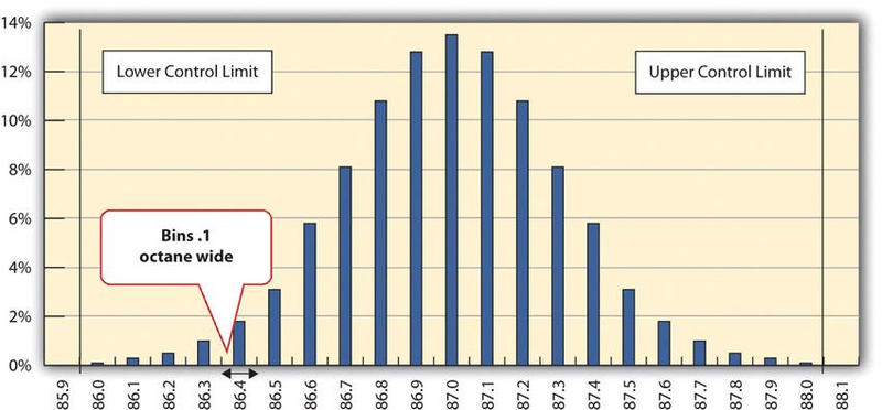
Figure 14.1 Normal Distribution of Measurements shows that the most common measurements of octane rating are close to 87 and that the other measurements are distributed equally above and below 87. The shape of the distribution chart supports the central limit theorem’s assumption that the factors that are affecting the octane rating are random and tend to offset each other, which is indicated by the symmetric shape. This distribution is a classic example of a normal distribution. The quality control manager notices that none of the measurements are above 88 or below 86 so they are within control limits, and she concludes that the process is working satisfactorily.
Example: Standard Deviation of Gasoline Samples
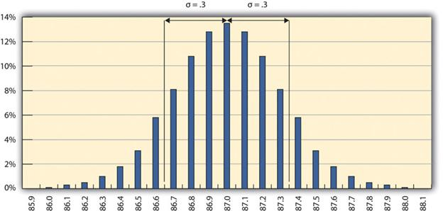
The refinery’s quality control manager uses the standard deviation function in her spreadsheet program to find the standard deviation of the sample measurements and finds that for her data, the standard deviation is 0.3 octane. She marks the range on the frequency distribution chart to show the values that fall within one sigma (standard deviation) on either side of the mean (Figure 14.2 One Sigma Range Most of the measurements are within 0.3 octane of 87. ).
For normal distributions, about 68.3% of the measurements fall within one standard deviation on either side of the mean. This is a useful rule of thumb for analyzing some types of data. If the variation between measurements is caused by random factors that result in a normal distribution, and someone tells you the mean and the standard deviation, you know that a little over two-thirds of the measurements are within a standard deviation on either side of the mean. Because of the shape of the curve, the number of measurements within two standard deviations is 95.4%, and the number of measurements within three standard deviations is 99.7%. For example, if someone said the average (mean) height for adult men in the United States is 178 cm (70 inches) and the standard deviation is about 8 cm (3 inches), you would know that 68% of the men in the United States are between 170 cm (67 inches) and 186 cm (73 inches) in height. You would also know that about 95% of the adult men in the United States were between 162 cm (64 inches) and 194 cm (76 inches) tall, and that almost all of them (99.7%) are between 154 cm (61 inches) and 202 cm (79 inches) tall. These figures are referred to as the 68-95-99.7 rule.
Example: Gasoline Within Three Standard Deviations
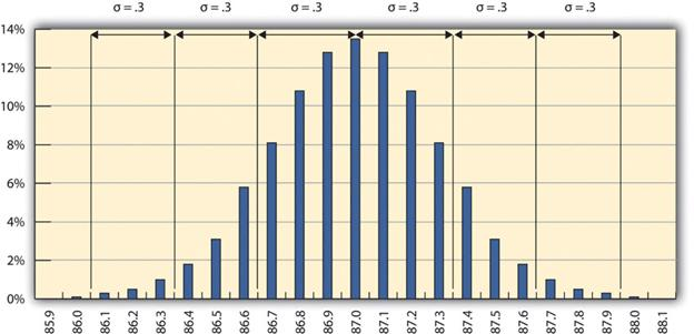
The refinery’s quality control manager marks the ranges included within two and three standard deviations, as shown in Figure 14.3 The 68-95-99.7 Rule . Some products must have less variability than others to meet their purpose. For example, if training designed to operate highly specialized and potentially dangerous machinery was assessed for quality, most participants would be expected to exceed the acceptable pass rate. Three standard deviations from the control limits might be fine for some products but not for others. In general, if the mean is six standard deviations from both control limits, the like lihood of a part exceeding the control limits from random variation is practically zero (2 in 1,000,000,000).
Example: A Step Project Improves Quality of Gasoline
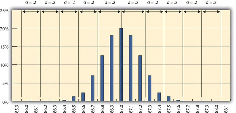
A new refinery process is installed that produces fuels with less variability. The refinery’s quality control manager takes a new set of samples and charts a new frequency distribution diagram, as shown in Figure 14.4 Smaller Standard Deviation .The refinery’s quality control manager calculates that the new standard deviation is 0.2 octane. From this, she can use the 68-95-99.7 rule to estimate that 68.3% of the fuel produced will be between 86.8 and 87.2 and that 99.7% will be between 86.4 and 87.6 octane. A shorthand way of describing this amount of control is to say that it is a five-sigma production system, which refers to the five standard deviations between the mean and the control limit on each side.
- 3364 reads
