


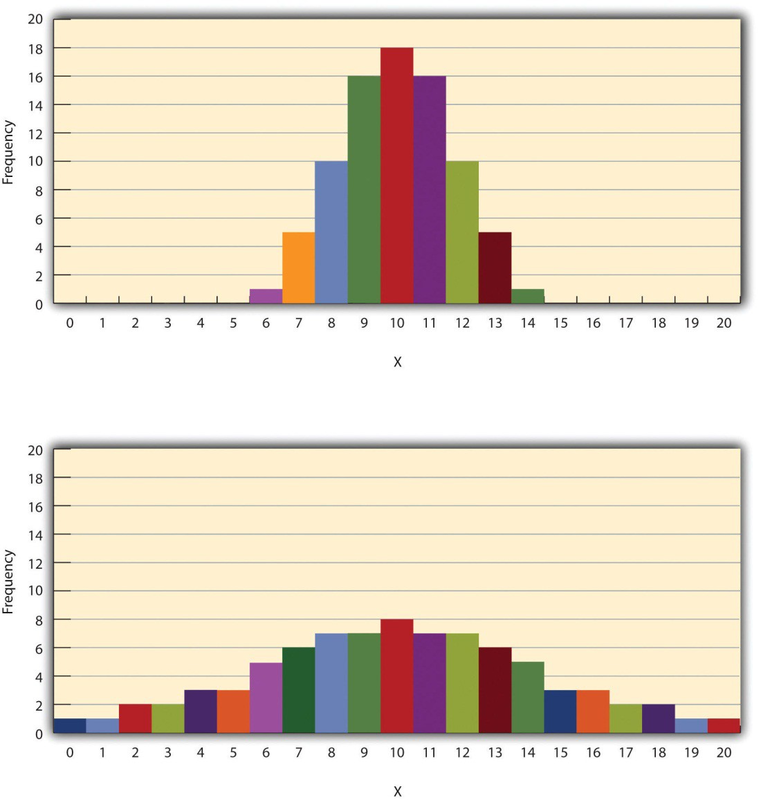
The variability of a distribution is the extent to which the scores vary around their central tendency. Consider the two distributions in Figure 12.4, both of which have the same central tendency. The mean, median, and mode of each distribution are 10. Notice, however, that the two distributions differ in terms of their variability. The top one has relatively low variability, with all the scores relatively close to the center. The bottom one has relatively high variability, with the scores are spread across a much greater range.
One simple measure of variability is the range, which is simply the difference between the highest and lowest scores in the distribution. The range of the self-esteem scores in Table 12.1, for example, is the difference between the highest score (24) and the lowest score (15). That is, the range is 24 − 15 = 9. Although the range is easy to compute and understand, it can be misleading when there are outliers. Imagine, for example, an exam on which all the students scored between 90 and 100. It has a range of 10. But if there was a single student who scored 20, the range would increase to 80—giving the impression that the scores were quite variable when in fact only one student differed substantially from the rest.
By far the most common measure of variability is the standard deviation. The standard deviation of a distribution is, roughly speaking, the average distance between the scores and the mean. For example, the standard deviations of the distributions in Figure 12.4 are 1.69 for the top distribution and 4.30 for the bottom one. That is, while the scores in the top distribution differ from the mean by about 1.69 units on average, the scores in the bottom distribution differ from the mean by about 4.30 units on average.
Computing the standard deviation involves a slight complication. Specifically, it involves finding the difference between each score and the mean, squaring each difference, finding the mean of these squared differences, and finally finding the square root of that mean. The formula looks like this:
The computations for the standard deviation are illustrated for a small set of data in Table 12.3 Computations for the Standard Deviation. The first column is a set of eight scores that has a mean of 5. The second column is the difference between each score and the mean. The third column is the square of each of these differences. Notice that although the differences can be negative, the squared differences are always positive—meaning that the standard deviation is always positive. At the bottom of the third column is the mean of the squared differences, which is also called the variance (symbolized SD2).
Although the variance is itself a measure of variability, it generally plays a larger role in inferential statistics than in descriptive statistics. Finally, below the variance is the square root of the variance, which is the standard deviation.
| X | X-M |

|
| 3 | -2 | 4 |
| 5 | 0 | 0 |
| 4 | -11 | 1 |
| 2 | -3 | 9 |
| 7 | 2 | 4 |
| 6 | 1 | 1 |
| 5 | 0 | 0 |
| 8 | 3 | 9 |
| M-5 | SD2=288=3.50 | |
| SD=3.50---√=1.87 |
N or N− 1
If you have already taken a statistics course, you may have learned to divide the sum of the squared differences by N− 1 rather than by Nwhen you compute the variance and standard deviation. Why is this?
By definition, the standard deviation is the square root of the mean of the squared differences. This implies dividing the sum of squared differences by N, as in the formula just presented. Computing the standard deviation this way is appropriate when your goal is simply to describe the variability in a sample. And learning it this way emphasizes that the variance is in fact the meanof the squared differences—and the standard deviation is the square root of this mean.
However, most calculators and software packages divide the sum of squared differences by N− 1. This is because the standard deviation of a sample tends to be a bit lower than the standard deviation of the population the sample was selected from. Dividing the sum of squares by N− 1 corrects for this tendency and results in a better estimate of the population standard deviation. Because researchers generally think of their data as representing a sample selected from a larger population—and because they are generally interested in drawing conclusions about the population—it makes sense to routinely apply this correction.
- 3630 reads
