


The one-way ANOVA is used to compare the means of more than two samples (M1, M2…MG) in a between-subjects design. The null hypothesis is that all the means are equal in the population: µ1= µ2 =…= µG. The alternative hypothesis is that not all the means in the population are equal.
The test statistic for the ANOVA is called F. It is a ratio of two estimates of the population variance based on the sample data. One estimate of the population variance is called the mean squares between groups (MSB)and is based on the differences among the sample means.
The other is called the mean squares within groups (MSW)and is based on the differences among the scores within each group. The F statistic is the ratio of the MSB to the MSW and can therefore be expressed as follows:
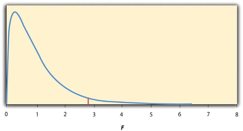
Again, the reason that F is useful is that we know how it is distributed when the null hypothesis is true. As shown in Figure 13.2, this distribution is unimodal and positively skewed with values
that cluster around 1. The precise shape of the distribution depends on both the number of groups and the sample size, and there is a degrees of freedom value associated with each of these. The
between- groups degrees of freedom is the number of groups minus one:  . The within-groups degrees of freedom is the total sample size minus the number of groups:
  . Again, knowing the distribution of F when the null hypothesis is true
allows us to find the p value.
. Again, knowing the distribution of F when the null hypothesis is true
allows us to find the p value.
The online tools in Descriptive Statistics and statistical software such as Excel and SPSS will compute Fand find the p value. If p is less than .05, then we reject the null hypothesis and conclude that there are differences among the group means in the population. If p is greater than .05, then we retain the null hypothesis and conclude that there is not enough evidence to say that there are differences. In the unlikely event that we would compute F by hand, we can use a table of critical values like Table 13.3 to make the decision. The idea is that any F ratio greater than the critical value has a p value of less than .05. Thus if the F ratio we compute is beyond the critical value, then we reject the null hypothesis. If the F ratio we compute is less than the critical value, then we retain the null hypothesis.
|
dfB |
|||
|
dfW |
2 |
3 |
4 |
|
8 |
4.459 |
4.066 |
3.838 |
|
9 |
4.256 |
3.863 |
3.633 |
|
10 |
4.103 |
3.708 |
3.478 |
|
11 |
3.982 |
3.587 |
3.357 |
|
12 |
3.885 |
3.490 |
3.259 |
|
13 |
3.806 |
3.411 |
3.179 |
|
14 |
3.739 |
3.344 |
3.112 |
|
15 |
3.682 |
3.287 |
3.056 |
|
16 |
3.634 |
3.239 |
3.007 |
|
17 |
3.592 |
3.197 |
2.965 |
|
18 |
3.555 |
3.160 |
2.928 |
|
19 |
3.522 |
3.127 |
2.895 |
|
20 |
3.493 |
3.098 |
2.866 |
|
21 |
3.467 |
3.072 |
2.840 |
|
22 |
3.443 |
3.049 |
2.817 |
|
23 |
3.422 |
3.028 |
2.796 |
|
24 |
3.403 |
3.009 |
2.776 |
|
25 |
3.385 |
2.991 |
2.759 |
|
30 |
3.316 |
2.922 |
2.690 |
|
35 |
3.267 |
2.874 |
2.641 |
|
40 |
3.232 |
2.839 |
2.606 |
|
45 |
3.204 |
2.812 |
2.579 |
|
50 |
3.183 |
2.790 |
2.557 |
|
55 |
3.165 |
2.773 |
2.540 |
|
60 |
3.150 |
2.758 |
2.525 |
|
65 |
3.138 |
2.746 |
2.513 |
|
70 |
3.128 |
2.736 |
2.503 |
|
75 |
3.119 |
2.727 |
2.494 |
|
80 |
3.111 |
2.719 |
2.486 |
|
85 |
3.104 |
2.712 |
2.479 |
|
90 |
3.098 |
2.706 |
2.473 |
|
95 |
3.092 |
2.700 |
2.467 |
|
100 |
3.087 |
2.696 |
2.463 |
- 3045 reads
