One-Sample Test

Available under Creative Commons-NonCommercial-ShareAlike 4.0 International License.

The one-sample t test is used to compare a sample mean (M) with a hypothetical population mean (μ0) that provides some interesting standard of comparison. The null hypothesis is that the mean for the population (µ) is equal to the hypothetical population mean: μ = μ0. The alternative hypothesis is that the mean for the population is different from the hypothetical population mean: μ ≠ μ0. To decide between these two hypotheses, we need to find the probability of obtaining the sample mean (or one more extreme) if the null hypothesis were true. But finding this pvalue requires first computing a test statistic called t. (A test statistic is a statistic that is computed only to help find the p value.) The formula for t is as follows:

Again, M is the sample mean and  is the hypothetical population mean of interest. SDis the sample standard deviation and Nis the sample size.

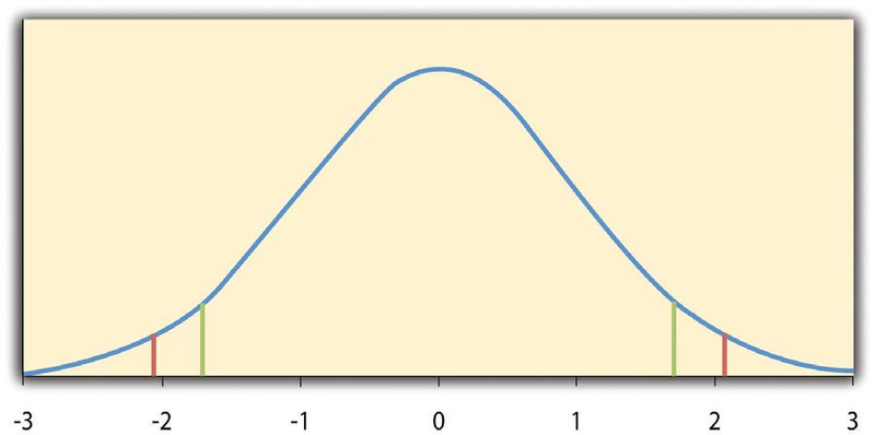
The reason the t statistic (or any test statistic) is useful is that we know how it is distributed when the null hypothesis is true. As shown in Figure 13.1, this distribution is unimodal and symmetrical, and it has a mean of 0. Its precise shape depends on a statistical concept called the degrees of freedom, which for a one-sample t test is N− 1. (There are 24 degrees of freedom for the distribution shown in Figure 13.1.) The important point is that knowing this distribution makes it possible to find the p value for any t score. Consider, for example, a t score of +1.50 based on a sample of 25. The probability of a t score at least this extreme is given by the proportion of t scores in the distribution that are at least this extreme. For now, let us define extreme as being far from zero in either direction. Thus the pvalue is the proportion of t scores that are +1.50 or above orthat are −1.50 or below—a value that turns out to be .14.

Figure 13.1 Distribution of t Scores (With 24 Degrees of Freedom) When the Null Hypothesis Is True 

The red vertical lines represent the two-tailed critical values, and the green vertical lines the one- tailed critical values when α = .05. 

 

Fortunately, we do not have to deal directly with the distribution of t scores. If we were to enter our sample data and hypothetical mean of interest into one of the online statistical tools in Descriptive Statistics or into a program like SPSS (Excel does not have a one-sample t test function), the output would include both the t score and the p value. At this point, the rest of the procedure is simple.

If p is less than .05, we reject the null hypothesis and conclude that the population mean differs from the hypothetical mean of interest. If p is greater than .05, we retain the null hypothesis and conclude that there is not enough evidence to say that the population mean differs from the hypothetical mean of interest. (Again, technically, we conclude only that we do not have enough evidence to conclude that it does differ.)

If we were to compute the t score by hand, we could use a table like Table 13.2 to make the decision. This table does not provide actual p values. Instead, it provides the critical values of t for different degrees of freedom (df) when α is .05. For now, let us focus on the two-tailed critical values in the last column of the table. Each of these values should be interpreted as a pair of values: one positive and one negative. For example, the two-tailed critical values when there are 24 degrees of freedom are +2.064 and −2.064. These are represented by the red vertical lines in Figure 13.1. The idea is that any t score below the lower critical value (the left-hand red line in Figure 13.1) is in the lowest 2.5% of the distribution, while any t score above the upper critical value (the right-hand red line) is in the highest 2.5% of the distribution. This means that any t score beyond the critical value in either direction is in the most extreme 5% of tscores when the null hypothesis is true and therefore has a p value less than .05. Thus if the t score we compute is beyond the critical value in either direction, then we reject the null hypothesis. If the tscore we compute is between the upper and lower critical values, then we retain the null hypothesis.

Thus far, we have considered what is called a two-tailed test, where we reject the null hypothesis if the t score for the sample is extreme in either direction. This makes sense when we believe that the sample mean might differ from the hypothetical population mean but we do not have good reason to expect the difference to go in a particular direction. But it is also possible to do a one-tailedtest, where we reject the null hypothesis only if the t score for the sample is extreme in one direction that we specify before collecting the data. This makes sense when we have good reason to expect the sample mean will differ from the hypothetical population mean in a particular direction.

Here is how it works. Each one-tailed critical value in Table 13.2 can again be interpreted as a pair of values: one positive and one negative. A t score below the lower critical value is in the lowest 5% of the distribution, and a tscore above the upper critical value is in the highest 5% of the distribution. For 24 degrees of freedom, these values are −1.711 and +1.711. (These are represented by the green vertical lines in Figure 13.1.) However, for a one-tailed test, we must decide before collecting data whether we expect the sample mean to be lower than the hypothetical population mean, in which case we would use only the lower critical value, or we expect the sample mean to be greater than the hypothetical population mean, in which case we would use only the upper critical value. Notice that we still reject the null hypothesis when the tscore for our sample is in the most extreme 5% of the t scores we would expect if the null hypothesis were true—so α remains at .05. We have simply redefined extreme to refer only to one tail of the distribution. The advantage of the one-tailed test is that critical values are less extreme. If the sample mean differs from the hypothetical population mean in the expected direction, then we have a better chance of rejecting the null hypothesis. The disadvantage is that if the sample mean differs from the hypothetical population mean in the unexpected direction, then there is no chance at all of rejecting the null hypothesis.