


Determining how well products meet grade requirements is done by taking measurements and then interpreting those measurements. Statistics—the mathematical interpretation of numerical data—is useful when interpreting large numbers of measurements and is used to determine how well the product meets a specification when the same product is made repeatedly. Measurements made on samples of the product must be between control limits—the upper and lower extremes of allowable variation—and it is up to management to design a process that will consistently produce products between those limits.
Setting Control Limits in Gasoline Production
A petroleum refinery produces large quantities of fuel in several grades. Samples of the fuels are extracted and measured at regular intervals. If a fuel is supposed to have an 87 octane performance, samples of the fuel should produce test results that are close to that value. Many of the samples will have scores that are different from 87. The differences are due to random factors that are difficult or expensive to control. Most of the samples should be close to the 87 rating and none of them should be too far off. The manufacturer has grades of 85 and 89, so they decide that none of the samples of the 87 octane fuel should be less than 86 or higher than 88.
If a process is designed to produce a product of a certain size or other measured characteristic, it is impossible to control all the small factors that can cause the product to differ slightly from the desired measurement. Some of these factors will produce products that have measurements that are larger than desired and some will have the opposite effect. If several random factors are affecting the process, they tend to offset each other most of the time, and the most common results are near the middle of the range. This idea is called the central limit theorem.
If the range of possible measurement values is divided equally into subdivisions called bins, the measurements can be sorted, and the number of measurements that fall into each bin can be counted. The result is a frequency distribution that shows how many measurements fall into each bin. If the effects that are causing the differences are random and tend to offset each other, the frequency distribution is called a normal distribution, which resembles the shape of a bell with edges that flare out. The edges of a theoretical normal distribution curve get very close to zero but do not reach zero.
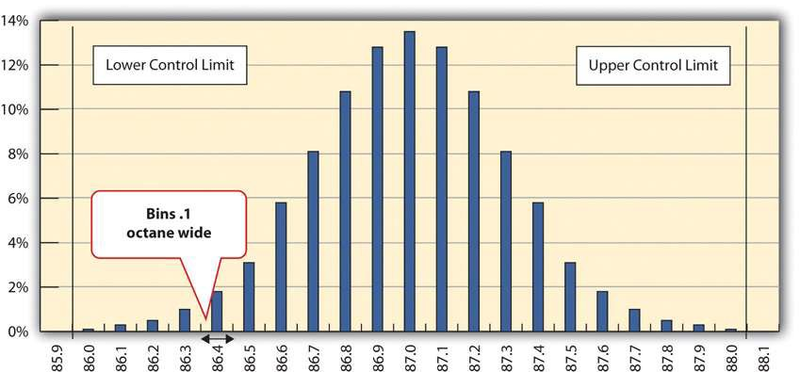
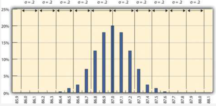
Normal Distribution of Gasoline Samples
A refinery’s quality control manager measures many samples of 87 octane gasoline, sorts the measurements by their octane rating into bins that are 0.1 octane wide, and then counts the number of measurements in each bin. Then she creates a frequency distribution chart of the data, as shown in Figure 10.1.
If the measurements of product samples are distributed equally above and below the center of the distribution as they are in Figure 10.1, the average of those measurements is also the center value that is called the mean and is represented in formulas by the lowercase Greek letter µ (pronounced mu). The amount of difference of the measurements from the central value is called the sample standard deviation or just the standard deviation. The first step in calculating the standard deviation is subtracting each measurement from the central value and then squaring that difference. (Recall from your mathematics courses that squaring a number is multiplying it by itself and that the result is always positive.) The next step is to sum these squared values and divide by the number of values minus one. The last step is to take the square root. The result can be thought of as an average difference. (If you had used the usual method of taking an average, the positive and negative numbers would have summed to zero.) Mathematicians represent the standard deviation with the lowercase Greek letter σ (pronounced sigma). If all the elements of a group are measured, it is called the standard deviation of the population and the second step does not use a minus one.
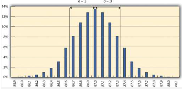
Standard Deviation of Gasoline Samples
The refinery’s quality control manager uses the standard deviation function in his spreadsheet program to find the standard deviation of the sample measurements and finds that for his data, the standard deviation is 0.3 octane. She marks the range on the frequency distribution chart to show the values that fall within one sigma (standard deviation) on either side of the mean. See Figure 10.2.
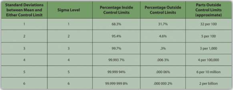
For normal distributions, about 68.3 percent of the measurements fall within one standard deviation on either side of the mean. This is a useful rule of thumb for analyzing some types of data. If the variation between measurements is caused by random factors that result in a normal distribution and someone tells you the mean and the standard deviation, you know that a little over two-thirds of the measurements are within a standard deviation on either side of the mean. Because of the shape of the curve, the number of measurements within two standard deviations is 95.4 percent, and the number of measurements within three standard deviations is 99.7 percent. For example, if someone said the average (mean) height for adult men in the United States is 5 feet 10 inches (70 inches) and the standard deviation is about 3 inches, you would know that 68 percent of the men in the United States are between five feet seven inches (67 inches) and six feet one inch (73 inches) in height. You would also know that about 95 percent of the adult men in the United States were between five feet four inches and six feet four inches tall, and that almost all of them (99.7 percent) are between five feet one inches and six feet seven inches tall. These figures are referred to as the 68-95-99.7 rule.
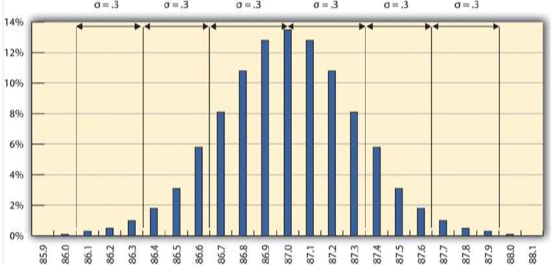
Almost All Samples of Gasoline are Within Three STD
The refinery’s quality control manager marks the ranges included within two and three standard deviations, as shown in Figure 10.3.
Some products must have less variability than others to meet their purpose. For example, if one machine drills a hole and another machine shapes a rod that will slide through the hole, it might be very important to be sure that if the smallest hole was ever matched with the widest rod, that the rod would still fit. Three standard deviations from the control limits might be fine for some products but not for others. In general, if the mean is six standard deviations from both control limits, the likelihood of a part exceeding the control limits from random variation is practically zero (2 in 1,000,000,000). Refer to Figure 10.4.
A Step Project Improves Quality of Gasoline
A new refinery process is installed that produces fuels with less variability. The refinery’s quality control manager takes a new set of samples and charts a new frequency distribution diagram, as shown in Figure 10.5.
The refinery’s quality control manager calculates that the new standard deviation is 0.2 octane. From this, he can use the 68-95-99.7 rule to estimate that 68.3 percent of the fuel produced will be between 86.8 and 87.2 and that 99.7 percent will be between 86.4 and 87.6 octane. A shorthand way of describing this amount of control is to say that it is a five-sigma production system, which refers to the five standard deviations between the mean and the control limit on each side.
KEY TAKEAWAYS
- Quality is the degree to which a product or service fulfills requirements and provides value for its price.
- Statistics is the mathematical interpretation of numerical data, and several statistical terms are used in quality control. Control limits are the boundaries of acceptable variation.
- If random factors cause variation, they will tend to cancel each other out—the central limit theorem. The central point in the distribution is the mean, which is represented by the Greek letter mu, µ. If you choose intervals called bins and count the number of samples that fall into each interval, the result is a frequency distribution. If you chart the distribution and the factors that cause variation are random, the frequency distribution is a normal distribution, which looks bell shaped.
- The center of the normal distribution is called the mean, and the average variation is calculated in a special way that finds the average of the squares of the differences between samples and the mean and then takes the square root. This average difference is called the standard deviation, which is represented by the Greek letter sigma, σ.
- About 68 percent of the samples are within one standard deviation, 95.4 percent are within two, and 99.7 percent are within three.
EXERCISES
- According to the ISO, quality is the degree to which a set of inherent characteristics fulfill .
- The upper and lower extremes of acceptable variation from the mean are called the limits.
- The odds that a sample’s measurement will be within one standard deviation of the mean is percent.
- How is quality related to grade?
- If the measurements in a frequency distribution chart are grouped near the mean in normal distribution, what does that imply about the causes of the variation?
- If you have a set of sample data and you had to calculate the standard deviation, what are the steps?
- If a set of sample measurements has a mean of 100, a normal distribution, a standard deviation of 2, and control limits of 94 and 106, what percentage of the samples are expected to be between 94 and 106? Explain your answer.
Using Statistical Measures
Choose two groups of people or items that have a measurable characteristic that can be compared, such as the height of adult males and females. Describe the distribution of the measurements by stating whether you think the groups have a relatively small or large standard deviation and whether the distributions overlap (e.g., some women are taller than some men even though the mean height for men is greater than the mean height for women). Demonstrate that you know how to use the following terms correctly in context:
- Normal distribution
- Standard deviation
- Mean
- 3087 reads
