


Even though Joan is an economist, her knowledge of the market for jewelry boxes was based on experience and insight. She understands the market because she has bought and sold jewelry boxes and their raw materials and she has built them from scratch. Joan decided she should put some of her economics training to work and determine the ideal price and quantity to sell that would generate the most profit.
The typical demand curve has the price on the y-axis and the quantity demanded on the x-axis and is downward-sloping. 1 A demand curve can be represented as a linear mathematical formula with quantity as the dependent variable (q = −5p + 400) or with price as the dependent variable (p = −5q + 80). A demand curve is a very useful diagram for describing the relationship between the price level and the quantity demanded at each price level. In general, as the price of a product increases, the demand for the good decreases. Similarly, as the price of a product decreases, the demand for the good increases. This section discusses how the demand curve can be used to identify the optimal price and quantity for selling just one version of a product.
Since Joan is a near-monopoly working in a market characterized by monopolistic competition, she can set her variable costs and fixed costs within certain limits related to the features she has established for her Jewelry boxes. Joan used algebra to come up with the optimal selling price for her standard jewelry box. This is the price that generates the greatest profit given the $15 variable costs and the $2,000 fixed costs.
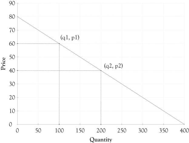
Her first task was to develop a demand equation. The demand equation relates the quantity of the good demanded by consumers to the price of the good. Demand equations are in the form: Price = constant + slope*Quantity. This can be calculated by finding the slope of the curve using any two points (see Figure 3.9). We will use the points (q1, p1) or (100, $60) and (q2, p2) or (200, $40). The slope is the rise over the run or:
Slope = (60 − 40)/ (100 − 200)
Slope = 20/−100
Slope = −0.2
The constant is calculated by determining where the demand line crosses the y-axis or, in this situation, the price or P-axis. This is accomplished by using the point slope form of the demand equation and any point such as (100, $60). The resulting constant is 80.
p − p1 = slope(q − q1)
p − 60 = −0.2(q − 100)
p = 60 + 0.2q + 20
p = 80 − 0.2q
In many instances, the demand curve is expressed in terms of p because the price determines the amount demanded. You can just substitute a price into the following formula and find out how many units will be sold.
q = −5p + 400
So if Joan decides to price each box at $50, then she will be able to sell 150 units.
Now that the demand equation has been found (p = −0.2q + 80 or q = −5p + 400), Joan’s next step was to determine the quantity where profits are maximized. This is accomplished by identifying where marginal revenue equals marginal cost. This is completed in two steps. The first step is to substitute the demand curve equation into the total revenue equation in order to get the total revenue calculation in terms of the quantity sold or q.
p = 80 − 0.2q
Total revenue = p × q
Total revenue = (80 − 0.2q) × q
Total revenue = 80q − 0.2q2
The above equation can be used to express the total revenue as a function of the quantity produced. We can check this answer by substituting 200 into the total revenue equation. For example, the total revenue when production is 200 units would be 80 × 200 − 0.2 × 2002 or $8,000. This is the same value for total revenue using the p × q equation for total revenue ($40 × 200 = $8,000).
The second step is to find the quantity where marginal cost equals marginal revenue. This is accomplished by taking the first derivative of the total revenue equation with respect to q. This is then set to the marginal cost and then solved for q. The marginal cost is actually the variable cost in this example. The marginal cost to produce one additional jewelry box is $15.
Total revenue = 80q − 0.2q2
Marginal revenue = dtr/dq = 80 − 0.4q
Marginal revenue = Marginal cost
80 − 0.4q = 15
−0.4q = −65
q = 162.5
The 162.5 quantity is rounded up to 163 and then substituted into the p = 80 − 0.2q equation.
p = 80 − 0.2(163)
p = 47.4
The 47.4 price was rounded down to $47. This is the short-term optimal revenue solution.
Profit = $47 × 163 − $15 × 163 − $2,000
Profit = $3,216
Joan decided after her analysis to produce fewer jewelry boxes since she could make more money selling fewer boxes at a higher price. She could have done a similar analysis using spreadsheet software and come up with a similar solution. She would, however, still need the original demand function along with an understanding of her variable and fixed costs to produce the jewelry boxes.
- 12006 reads
