


Available under Creative Commons-ShareAlike 4.0 International License.
Edited script contains the plot commands:
% This script uses readings from a Tensile test and
% Computes Strain and Stress values
clc % Clear screen
disp('This script uses readings from a Tensile test and')
disp('Computes Strain and Stress values')
disp(' ') % Display a blank line
Specimen_dia=12.7; % Specimen diameter in mm
% Load in kN
Load_kN=[0;4.89;9.779;14.67;19.56;24.45;...
27.62;29.39;32.68;33.95;34.58;35.22;...
35.72;40.54;48.39;59.03;65.87;69.42;...
69.67;68.15;60.81];
% Gage length in mm
Length_mm=[50.8;50.8102;50.8203;50.8305;...
50.8406;50.8508;50.8610;50.8711;...
50.9016;50.9270;50.9524;50.9778;...
51.0032;51.816;53.340;55.880;58.420;...
60.96;61.468;63.5;66.04];
% Calculate x-sectional area im m2
Cross_sectional_Area=pi/4*((Specimen_dia/1000)^2);
% Calculate change in length, initial lenght is 50.8 mm
Delta_L=Length_mm-50.8;
% Calculate Stress in MPa
Sigma=(Load_kN./Cross_sectional_Area)*10^(-3);
% Calculate Strain in mm/mm
Epsilon=Delta_L./50.8;
str = ['Specimen diameter is ', num2str(Specimen_dia), ' mm.'];
disp(str);
Results=[Load_kN Length_mm Delta_L Sigma Epsilon];
% Tabulated results
disp(' Load Length Delta L Stress Strain')
disp(Results)
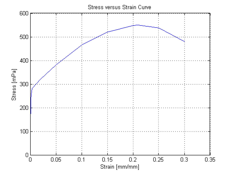
% Plot Stress versus Strain
plot(Epsilon,Sigma)
title('Stress versus Strain Curve')
xlabel('Strain [mm/mm]')
ylabel('Stress [mPa]')
grid
In addition to Command Window output, the following plot is generated:
- 瀏覽次數:1967
