


Given the following data, plot an x-y graph and determine the area under a curve between x=3 and x=30
|
Index |
x [m] |
y [N] |
|
1 |
3 |
27.00 |
|
2 |
10 |
14.50 |
|
3 |
15 |
9.40 |
|
4 |
20 |
6.70 |
|
5 |
25 |
5.30 |
|
6 |
30 |
4.50 |
First, let us enter the data set. For x, issue the following command x=[3,10,15,20,25,30];. And for y, y=[27,14.5,9.4,6.7,5.3,4.5];. If yu type in [x',y'], you will see the following tabulated result. Here we transpose row vectors with ’ and displaying them as columns:
ans =

 3.0000 27.0000
10.0000 14.5000
15.0000  9.4000
20.0000  6.7000
25.0000  5.3000
30.0000  4.5000
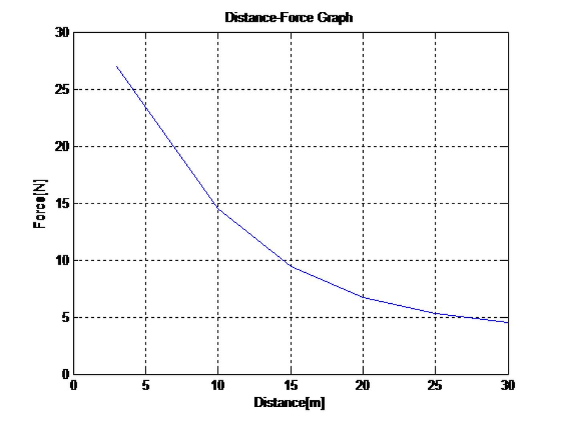
Compare the data set above with the given information in the question (Table 6.1). To plot the data type the following:
plot(x,y),title('Distance-Force Graph'),xlabel('Distance[m]'),ylabel('Force[N]'),grid
The following figure is generated:
To compute dx for consecutive x values, we will use the index for each x value, see the given data in the question (Table 6.1).:
dx=[x(2)-x(1),x(3)-x(2),x(4)-x(3),x(5)-x(4),x(6)-x(5)];
dy is computed by the following command:
dy=[0.5*(y(2)+y(1)),0.5*(y(3)+y(2)),0.5*(y(4)+y(3)),0.5*(y(5)+y(4)),0.5*(y(6)+y(5))];
dx and dy can be displayed with the following command: [dx',dy']. The result will look like this:
    [dx',dy']

ans =

    7.0000  20.7500
    5.0000  11.9500
    5.0000   8.0500
    5.0000   6.0000
    5.0000   4.9000
Our results so far are shown below
|
x [m] |
y [N] |
dx [m] |
dy [N] |
|
3 |
27.00 |
||
|
10 |
14.50 |
7.00 |
20.75 |
|
15 |
9.40 |
5.00 |
11.95 |
|
20 |
6.70 |
5.00 |
8.05 |
|
25 |
5.30 |
5.00 |
6.00 |
|
30 |
4.50 |
5.00 |
4.90 |
If we multiply dx by dy, we find da for each element under the curve. The differential area da=dx*dy, can be computed using the ’term by term multiplication’ technique in MATLAB as follows:
    da=dx.*dy
da =
    145.2500 59.7500 40.2500 30.0000 24.5000
Each value above represents an element under the curve or the area of trapezoid. By taking the sum of array elements, we find the total area under the curve.
    sum(da)
ans =
    299.7500
The following (Table 6.3) illustrates all the steps and results of our MATLAB computation.
|
x [m] |
y [N] |
dx [m] |
dy [N] |
dA [Nm] |
|
3 |
27.00 |
|||
|
10 |
14.50 |
7.00 |
20.75 |
145.25 |
|
15 |
9.40 |
5.00 |
11.95 |
59.75 |
|
20 |
6.70 |
5.00 |
8.05 |
40.25 |
|
25 |
5.30 |
5.00 |
6.00 |
30.00 |
|
30 |
4.50 |
5.00 |
4.90 |
24.50 |
|
299.75 |
- 瀏覽次數:2667
