


Since Accounting Depreciation attempts to capture a real economic phenomenon, it must be based on economic reasoning. It is not a mechanical procedure or an arithmetic exercise. The prevailing concern when determining depreciation methodology should not be to "guess" the correct depreciation rate, but to estimate reasonably the useful life of the asset under depreciation in time-units, and then calculate the corresponding depreciation rate that will result in extinguishing the value of the asset from the books when the estimated useful life ends too, given the Depreciation method chosen.
In the Straight-Line method, the mapping of Useful Life to Depreciation Rate is easy. If "x" is the estimated useful life, say in years, then the Yearly Depreciation Rate "d" is d = 1/x. For example, if you expect that the company will use a vehicle for 10 years, then the Yearly Depreciation Rate for this vehicle is 1/10 = 0,1 = 10%, under the Straight-line method.
In the Declining Balance Method, things are trickier. First we must note that from a mathematical point of view, the value of the asset is never fully extinguished under the Declining Balance method, but it approaches arbitrarily close to zero. In practice, companies that use the Declining Balance Method, decide on a "materiality threshold" for the non-depreciated (residual) value of the asset, usually up to 10% of its initial purchase value. Essentially then, they calculate the depreciation rate which, under the Declining Balance method, will extinguish the largest part of the Value of the asset (i.e. 90% or 95%) at the end of its economic useful life. When they reach that point in time, they depreciate what's left in the next accounting period.
Now, the Declining Balance method is expressed as a Difference Equation. Denote "d" the depreciation rate, "r" the remaining value at the end of the estimated useful life, as a percentage of initial purchase value (=> 0 < r < 1) and V(t) the nondepreciated value of the asset at the end of period t. Denote also "n" the useful life of the asset, say in years. Then you have

Going backwards in the Difference equation and writing for period "n" you get
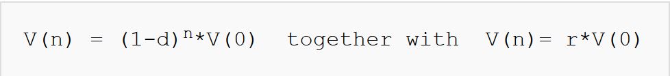
Solving together the two equations you get
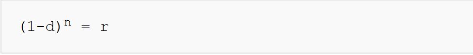
So we see that by estimating the useful life of the asset (the "n"), and given that we have chosen a residual value (the "r", as a percentage of the initial purchase value of the asset), we can uniquely determine the required depreciation rate "d" to use in our depreciation calculations so that our accounting books reflect, at least approximately, what happens in actual economic activity.
- 3409 reads
