


The transport layer must deal with the imperfections of the network layer service. There are three types of imperfections that must be considered by the transport layer :
- Segments can be corrupted by transmission errors
- Segments can be lost
- Segments can be reordered or duplicated
To deal with these types of imperfections, transport protocols rely on different types of mechanisms. The first problem is transmission errors. The segments sent by a transport entity is processed by the network and datalink layers and finally transmitted by the physical layer. All of these layers are imperfect. For example, the physical layer may be affected by different types of errors :
- random isolated errors where the value of a single bit has been modified due to a transmission error
- random burst errors where the values of n consecutive bits have been changed due to transmission errors
- random bit creations and random bit removals where bits have been added or removed due to transmission errors
The only solution to protect against transmission errors is to add redundancy to the segments that are sent. Information Theory defines two mechanisms that can be used to transmit information over a transmission channel affected by random errors. These two mechanisms add redundancy to the information sent, to allow the receiver to detect or sometimes even correct transmission errors. A detailed discussion of these mechanisms is outside the scope of this chapter, but it is useful to consider a simple mechanism to understand its operation and its limitations.
Information theory defines coding schemes. There are different types of coding schemes, but let us focus on coding schemes that operate on binary strings. A coding scheme is a function that maps information encoded as a string of m bits into a string of n bits. The simplest coding scheme is the even parity coding. This coding scheme takes an m bits source string and produces an m+1 bits coded string where the first m bits of the coded string are the bits of the source string and the last bit of the coded string is chosen such that the coded string will always contain an even number of bits set to 1. For example :
- 1001 is encoded as 10010
- 1101 is encoded as 11011
This parity scheme has been used in some RAMs as well as to encode characters sent over a serial line. It is easy to show that this coding scheme allows the receiver to detect a single transmission error, but it cannot correct it. However, if two or more bits are in error, the receiver may not always be able to detect the error.
Some coding schemes allow the receiver to correct some transmission errors. For example, consider the coding scheme that encodes each source bit as follows :
- 1 is encoded as 111
- 0 is encoded as 000
This simple coding scheme forces the sender to transmit three bits for each source bit. However, it allows the receiver to correct single bit errors. More advanced coding systems that allow to recover from errors are used in several types of physical layers.
Transport protocols use error detection schemes, but none of the widely used transport protocols rely on error correction schemes. To detect errors, a segment is usually divided into two parts :
- a header that contains the fields used by the transport protocol to ensure reliable delivery. The header contains a checksum or Cyclical Redundancy Check (CRC) [Williams1993] that is used to detect transmission errors
- a payload that contains the user data passed by the application layer.
Some segment headers also include a length , which indicates the total length of the segment or the length of the payload.
The simplest error detection scheme is the checksum. A checksum is basically an arithmetic sum of all the bytes that a segment is composed of. There are different types of checksums. For example, an eight bit checksum can be computed as the arithmetic sum of all the bytes of (both the header and trailer of) the segment. The checksum is computed by the sender before sending the segment and the receiver verifies the checksum upon reception of each segment. The receiver discards segments received with an invalid checksum. Checksums can be easily implemented in software, but their error detection capabilities are limited. Cyclical Redundancy Checks (CRC) have better error detection capabilities [SGP98], but require more CPU when implemented in software.
Most of the protocols in the TCP/IP protocol suite rely on the simple Internet checksum in order to verify that the received segment has not been affected by transmission errors. Despite its popularity and ease of implementation, the Internet checksum is not the only available checksum mechanism. Cyclical Redundancy Checks (CRC) are very powerful error detection schemes that are used notably on disks, by many datalink layer protocols and file formats such as zip or png. They can easily be implemented efficiently in hardware and have better error-detection capabilities than the Internet checksum [SGP98] . However, when the first transport protocols were designed, CRCs were considered to be too CPU-intensive for software implementations and other checksum mechanisms were used instead. The TCP/IP community chose the Internet checksum, the OSI community chose the Fletcher checksum [Sklower89] . Now, there are efficient techniques to quickly compute CRCs in software [Feldmeier95] , the SCTP protocol initially chose the Adler-32 checksum but replaced it recently with a CRC (see RFC 3309).
The second imperfection of the network layer is that segments may be lost. As we will see later, the main cause of packet losses in the network layer is the lack of buffers in intermediate routers. Since the receiver sends an acknowledgement segment after having received each data segment, the simplest solution to deal with losses is to use a retransmission timer. When the sender sends a segment, it starts a retransmission timer. The value of this retransmission timer should be larger than the round-trip-time, i.e. the delay between the transmission of a data segment and the reception of the corresponding acknowledgement. When the retransmission timer expires, the sender assumes that the data segment has been lost and retransmits it. This is illustrated in the figure below.
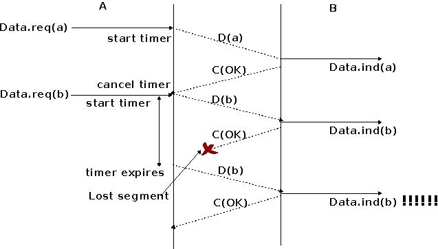
Unfortunately, retransmission timers alone are not sufficient to recover from segment losses. Let us consider, as an example, the situation depicted below where an acknowledgement is lost. In this case, the sender retransmits
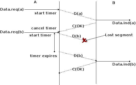
the data segment that has not been acknowledged. Unfortunately, as illustrated in the figure below, the receiver considers the retransmission as a new segment whose payload must be delivered to its user.
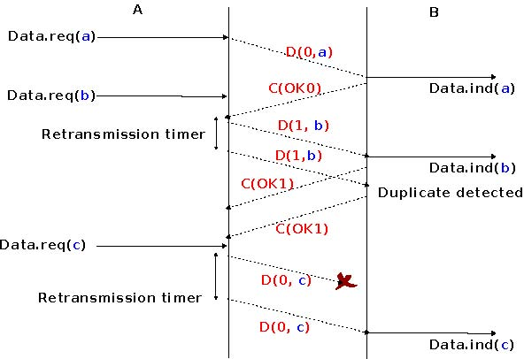
To solve this problem, transport protocols associate a sequence number to each data segment. This sequence number is one of the fields found in the header of data segments. We use the notation D(S,...) to indicate a data segment whose sequence number field is set to S. The acknowledgements also contain a sequence number indicating the data segments that it is acknowledging. We use OKS to indicate an acknowledgement segment that confirms the reception of D(S,...). The sequence number is encoded as a bit string of fixed length. The simplest transport protocol is the Alternating Bit Protocol (ABP).
The Alternating Bit Protocol uses a single bit to encode the sequence number. It can be implemented easily. The sender and the receivers only require a four states Finite State Machine.
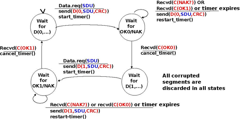
The initial state of the sender is Wait for D(0,...). In this state, the sender waits for a Data.request. The first data segment that it sends uses sequence number 0. After having sent this segment, the sender waits for an OK0 acknowledgement. A segment is retransmitted upon expiration of the retransmission timer or if an acknowledgement with an incorrect sequence number has been received.
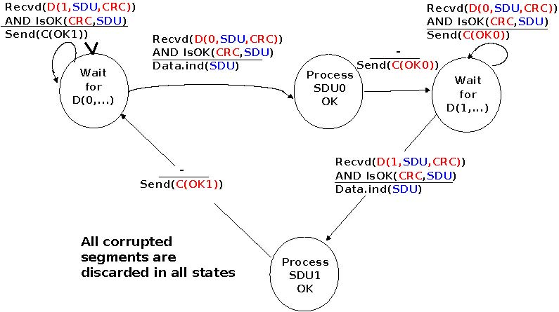
The receiver first waits for D(0,...). If the segment contains a correct CRC, it passes the SDU to its user and sends OK0. If the segment contains an invalid CRC, it is immediately discarded. Then, the receiver waits for D(1,...). In this state, it may receive a duplicate D(0,...) or a data segment with an invalid CRC. In both cases, it returns an OK0 segment to allow the sender to recover from the possible loss of the previous OK0 segment.
The receiver FSM of the Alternating bit protocol discards all segments that contain an invalid CRC. This is the safest approach since the received segment can be completely different from the segment sent by the remote host. A receiver should not attempt at extracting information from a corrupted segment because it cannot know which portion of the segment has been affected by the error.
The figure below illustrates the operation of the alternating bit protocol.
The Alternating Bit Protocol can recover from transmission errors and segment losses. However, it has one important drawback. Consider two hosts that are directly connected by a 50 Kbits/sec satellite link that has a 250 milliseconds propagation delay. If these hosts send 1000 bits segments, then the maximum throughput that can be achieved by the alternating bit protocol is one segment every 20+250+250 = 520 milliseconds if we ignore the transmission time of the acknowledgement. This is less than 2 Kbits/sec !
Go-back-n and selective repeat
To overcome the performance limitations of the alternating bit protocol, transport protocols rely on pipelining. This technique allows a sender to transmit several consecutive segments without being forced to wait for an acknowledgement after each segment. Each data segment contains a sequence number encoded in an n bits field.
Pipelining allows the sender to transmit segments at a higher rate, but we need to ensure that the receiver does not
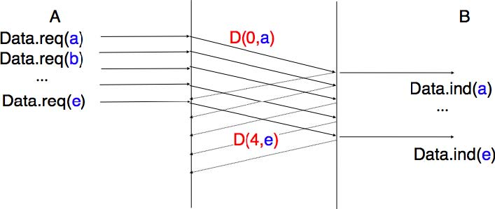
become overloaded. Otherwise, the segments sent by the sender are not correctly received by the destination. The transport protocols that rely on pipelining allow the sender to transmit W unacknowledged segments before being forced to wait for an acknowledgement from the receiving entity.
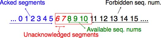
This is implemented by using a sliding window. The sliding window is the set of consecutive sequence numbers that the sender can use when transmitting segments without being forced to wait for an acknowledgement. The figure below shows a sliding window containing five segments (6,7,8,9 and 10). Two of these sequence numbers (6 and 7) have been used to send segments and only three sequence numbers (8, 9 and 10) remain in the sliding window. The sliding window is said to be closed once all sequence numbers contained in the sliding window have been used.
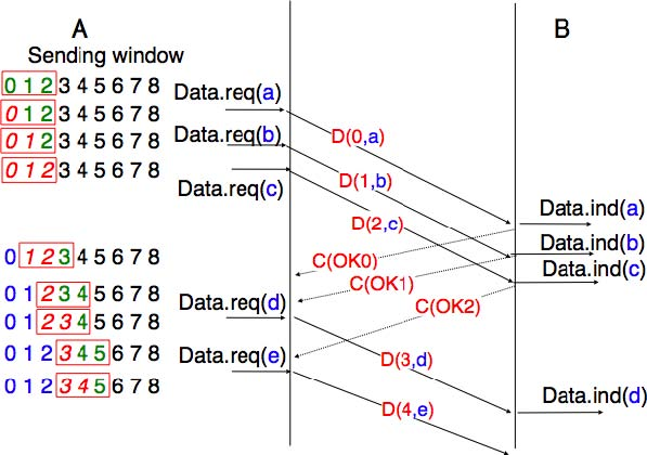
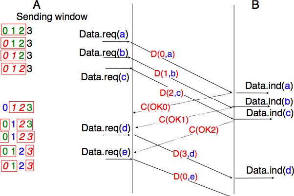
The figure below illustrates the operation of the sliding window. The sliding window shown contains three segments. The sender can thus transmit three segments before being forced to wait for an acknowledgement. The sliding window moves to the higher sequence numbers upon reception of acknowledgements. When the first acknowledgement (OK0) is received, it allows the sender to move its sliding window to the right and sequence number 3 becomes available. This sequence number is used later to transmit SDU d.
In practice, as the segment header encodes the sequence number in an n bits string, only the sequence numbers between 0 and 2n − 1 can be used. This implies that the same sequence number is used for different segments and that the sliding window will wrap. This is illustrated in the figure below assuming that 2 bits are used to encode the sequence number in the segment header. Note that upon reception of OK1, the sender slides its window and can use sequence number 0 again.
Unfortunately, segment losses do not disappear because a transport protocol is using a sliding window. To recover from segment losses, a sliding window protocol must define :
- a heuristic to detect segment losses
- a retransmission strategy to retransmit the lost segments.
The simplest sliding window protocol uses go-back-n recovery. Intuitively, go-back-n operates as follows. A go-back-n receiver is as simple as possible. It only accepts the segments that arrive in-sequence. A go-back-n receiver discards any out-of-sequence segment that it receives. When go-back-n receives a data segment, it always returns an acknowledgement containing the sequence number of the last in-sequence segment that it has received. This acknowledgement is said to be cumulative. When a go-back-n receiver sends an acknowledgement for sequence number x, it implicitly acknowledges the reception of all segments whose sequence number is earlier than x. A key advantage of these cumulative acknowledgements is that it is easy to recover from the loss of an acknowledgement. Consider for example a go-back-n receiver that received segments 1, 2 and 3. It sent OK1, OK2 and OK3. Unfortunately, OK1 and OK2 were lost. Thanks to the cumulative acknowledgements, when the receiver receives OK3, it knows that all three segments have been correctly received.
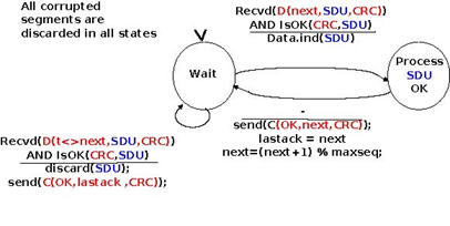
The figure below shows the FSM of a simple go-back-n receiver. This receiver uses two variables : lastack and next. next is the next expected sequence number and lastack the sequence number of the last data segment that has been acknowledged. The receiver only accepts the segments that are received in sequence. maxseq is the number of different sequence numbers (2n).
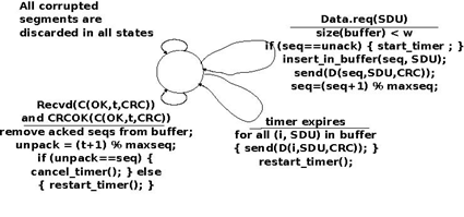
A go-back-n sender is also very simple. It uses a sending buffer that can store an entire sliding window of segments 1. The segments are sent with increasing sequence number (modulo maxseq). The sender must wait for an acknowledgement once its sending buffer is full. When a go-back-n sender receives an acknowledgement, it removes from the sending buffer all the acknowledged segments and uses a retransmission timer to detect segment losses. A simple go-back-n sender maintains one retransmission timer per connection. This timer is started when the first segment is sent. When the go-back-n sender receives an acknowledgement, it restarts the retransmission timer only if there are still unacknowledged segments in its sending buffer. When the retransmission timer expires, the go-back-n sender assumes that all the unacknowledged segments currently stored in its sending buffer have been lost. It thus retransmits all the unacknowledged segments in the buffer and restarts its retransmission timer.
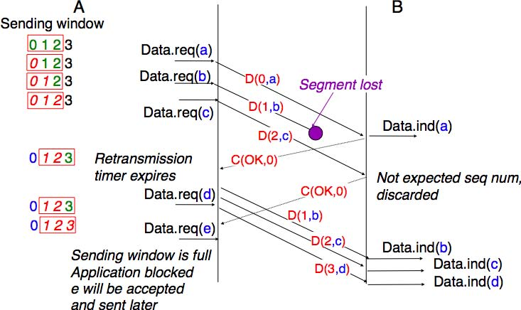
The operation of go-back-n is illustrated in the figure below. In this figure, note that upon reception of the outof-sequence segment D(2,c), the receiver returns a cumulative acknowledgement C(OK,0) that acknowledges all the segments that have been received in sequence. The lost segment is retransmitted upon the expiration of the retransmission timer.
The main advantage of go-back-n is that it can be easily implemented, and it can also provide good performance when only a few segments are lost. However, when there are many losses, the performance of go-back-n quickly drops for two reasons :
- the go-back-n receiver does not accept out-of-sequence segments
- the go-back-n sender retransmits all unacknowledged segments once its has detected a loss
Selective repeat is a better strategy to recover from segment losses. Intuitively, selective repeat allows the receiver to accept out-of-sequence segments. Furthermore, when a selective repeat sender detects losses, it only retransmits the segments that have been lost and not the segments that have already been correctly received.
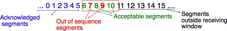
A selective repeat receiver maintains a sliding window of W segments and stores in a buffer the out-of-sequence segments that it receives. The figure below shows a five segment receive window on a receiver that has already received segments 7 and 9.
A selective repeat receiver discards all segments having an invalid CRC, and maintains the variable lastack as the sequence number of the last in-sequence segment that it has received. The receiver always includes the value of lastack in the acknowledgements that it sends. Some protocols also allow the selective repeat receiver to acknowledge the out-of-sequence segments that it has received. This can be done for example by placing the list of the sequence numbers of the correctly received, but out-of-sequence segments in the acknowledgements together with the lastack value.
When a selective repeat receiver receives a data segment, it first verifies whether the segment is inside its receiving window. If yes, the segment is placed in the receive buffer. If not, the received segment is discarded and an acknowledgement containing lastack is sent to the sender. The receiver then removes all consecutive segments starting at lastack (if any) from the receive buffer. The payloads of these segments are delivered to the user, lastack and the receiving window are updated, and an acknowledgement acknowledging the last segment received in sequence is sent.
The selective repeat sender maintains a sending buffer that can store up to W unacknowledged segments. These segments are sent as long as the sending buffer is not full. Several implementations of a selective repeat sender are possible. A simple implementation is to associate a retransmission timer to each segment. The timer is started when the segment is sent and cancelled upon reception of an acknowledgement that covers this segment. When a retransmission timer expires, the corresponding segment is retransmitted and this retransmission timer is restarted. When an acknowledgement is received, all the segments that are covered by this acknowledgement are removed from the sending buffer and the sliding window is updated.
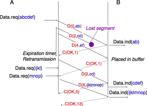
The figure below illustrates the operation of selective repeat when segments are lost. In this figure, C(OK,x) is used to indicate that all segments, up to and including sequence number x have been received correctly.
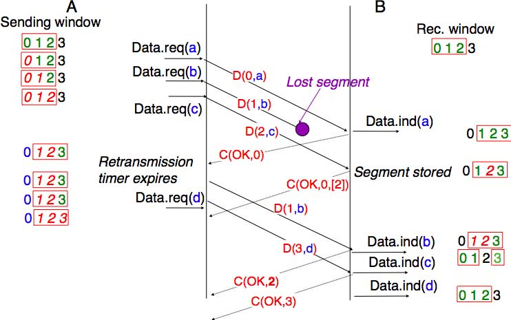
Pure cumulative acknowledgements work well with the go-back-n strategy. However, with only cumulative acknowledgements a selective repeat sender cannot easily determine which data segments have been correctly received after a data segment has been lost. For example, in the figure above, the second C(OK,0) does not inform explicitly the sender of the reception of D(2,c) and the sender could retransmit this segment although it has already been received. A possible solution to improve the performance of selective repeat is to provide additional information about the received segments in the acknowledgements that are returned by the receiver. For example, the receiver could add in the returned acknowledgement the list of the sequence numbers of all segments that have already been received. Such acknowledgements are sometimes called selective acknowledgements. This is illustrated in the figure below.
In the figure above, when the sender receives C(OK,0,[2]), it knows that all segments up to and including D(0,...) have been correctly received. It also knows that segment D(2,...) has been received and can cancel the retransmission timer associated to this segment. However, this segment should not be removed from the sending buffer before the reception of a cumulative acknowledgement (C(OK,2) in the figure above) that covers this segment.
A transport protocol that uses n bits to encode its sequence number can send up to 2n different segments. However, to ensure a reliable delivery of the segments, go-back-n and selective repeat cannot use a sending window of 2n segments. Consider first go-back-n and assume that a sender sends 2n segments. These segments are received in-sequence by the destination, but all the returned acknowledgements are lost. The sender will retransmit all segments and they will all be accepted by the receiver and delivered a second time to the user. It is easy to see that this problem can be avoided if the maximum size of the sending window is 2n − 1 segments. A similar problem occurs with selective repeat. However, as the receiver accepts out-of-sequence segments, a sending window of 2n − 1 segments is not sufficient to ensure a reliable delivery of all segments. It can be easily shown that to avoid this problem, a selective repeat sender cannot use a window that is larger than 2n/2 segments.
Go-back-n or selective repeat are used by transport protocols to provide a reliable data transfer above an unreliable network layer service. Until now, we have assumed that the size of the sliding window was fixed for the entire lifetime of the connection 2. In practice a transport layer entity is usually implemented in the operating system and shares memory with other parts of the system. Furthermore, a transport layer entity must support several (possibly hundreds or thousands) of transport connections at the same time. This implies that the memory which can be used to support the sending or the receiving buffer of a transport connection may change during the lifetime of the connection. Thus, a transport protocol must allow the sender and the receiver to adjust their window sizes.
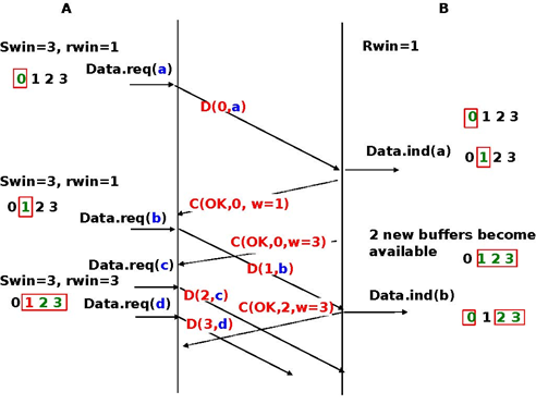
To deal with this issue, transport protocols allow the receiver to advertise the current size of its receiving window in all the acknowledgements that it sends. The receiving window advertised by the receiver bounds the size of the sending buffer used by the sender. In practice, the sender maintains two state variables : swin, the size of its sending window (that may be adjusted by the system) and rwin, the size of the receiving window advertised by the receiver. At any time, the number of unacknowledged segments cannot be larger than min(swin,rwin) 3. The utilisation of dynamic windows is illustrated in the figure below.
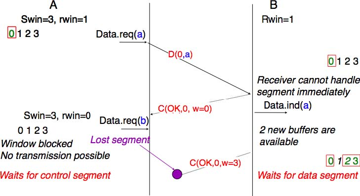
The receiver may adjust its advertised receive window based on its current memory consumption, but also to limit the bandwidth used by the sender. In practice, the receive buffer can also shrink as the application may not able to process the received data quickly enough. In this case, the receive buffer may be completely full and the advertised receive window may shrink to 0. When the sender receives an acknowledgement with a receive window set to 0, it is blocked until it receives an acknowledgement with a positive receive window. Unfortunately, as shown in the figure below, the loss of this acknowledgement could cause a deadlock as the sender waits for an acknowledgement while the receiver is waiting for a data segment.
To solve this problem, transport protocols rely on a special timer : the persistence timer. This timer is started by the sender whenever it receives an acknowledgement advertising a receive window set to 0. When the timer expires, the sender retransmits an old segment in order to force the receiver to send a new acknowledgement, and hence send the current receive window size.
To conclude our description of the basic mechanisms found in transport protocols, we still need to discuss the impact of segments arriving in the wrong order. If two consecutive segments are reordered, the receiver relies on their sequence numbers to reorder them in its receive buffer. Unfortunately, as transport protocols reuse the same sequence number for different segments, if a segment is delayed for a prolonged period of time, it might still be accepted by the receiver. This is illustrated in the figure below where segment D(1,b) is delayed.
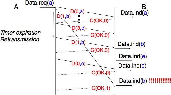
To deal with this problem, transport protocols combine two solutions. First, they use 32 bits or more to encode the sequence number in the segment header. This increases the overhead, but also increases the delay between the transmission of two different segments having the same sequence number. Second, transport protocols require the network layer to enforce a Maximum Segment Lifetime (MSL). The network layer must ensure that no packet remains in the network for more than MSL seconds. In the Internet the MSL is assumed 4 to be 2 minutes RFC793. Note that this limits the maximum bandwidth of a transport protocol. If it uses n bits to encode its sequence numbers, then it cannot send more than 2n segments every MSL seconds.
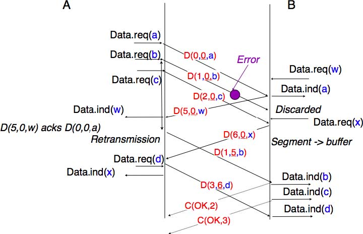
Transport protocols often need to send data in both directions. To reduce the overhead caused by the acknowledgements, most transport protocols use piggybacking. Thanks to this technique, a transport entity can place inside the header of the data segments that it sends, the acknowledgements and the receive window that it advertises for the opposite direction of the data flow. The main advantage of piggybacking is that it reduces the overhead as it is not necessary to send a complete segment to carry an acknowledgement. This is illustrated in the figure below where the acknowledgement number is underlined in the data segments. Piggybacking is only used when data flows in both directions. A receiver will generate a pure acknowledgement when it does not send data in the opposite direction as shown in the bottom of the figure.
The last point to be discussed about the data transfer mechanisms used by transport protocols is the provision of a byte stream service. As indicated in the first chapter, the byte stream service is widely used in the transport layer. The transport protocols that provide a byte stream service associate a sequence number to all the bytes that are sent and place the sequence number of the first byte of the segment in the segment’s header. This is illustrated in the figure below. In this example, the sender chooses to put two bytes in each of the first three segments. This is due to graphical reasons, a real transport protocol would use larger segments in practice. However, the division of the byte stream into segments combined with the losses and retransmissions explain why the byte stream service does not preserve the SDU boundaries.
Connection establishment and release
The last points to be discussed about the transport protocol are the mechanisms used to establish and release a transport connection.
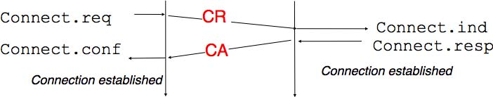
We explained in the first chapters the service primitives used to establish a connection. The simplest approach to establish a transport connection would be to define two special control segments : CR and CA. The CR segment is sent by the transport entity that wishes to initiate a connection. If the remote entity wishes to accept the connection, it replies by sending a CA segment. The transport connection is considered to be established once the CA segment has been received and data segments can be sent in both directions.
Unfortunately, this scheme is not sufficient for several reasons. First, a transport entity usually needs to maintain several transport connections with remote entities. Sometimes, different users (i.e. processes) running above a given transport entity request the establishment of several transport connections to different users attached to the same remote transport entity. These different transport connections must be clearly separated to ensure that data from one connection is not passed to the other connections. This can be achieved by using a connection identifier, chosen by the transport entities and placed inside each segment to allow the entity which receives a segment to easily associate it to one established connection.
Second, as the network layer is imperfect, the CR or CA segment can be lost, delayed, or suffer from transmission errors. To deal with these problems, the control segments must be protected by using a CRC or checksum to detect transmission errors. Furthermore, since the CA segment acknowledges the reception of the CR segment, the CR segment can be protected by using a retransmission timer.
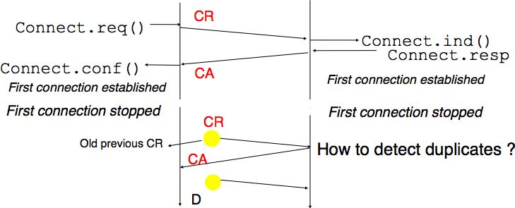
Unfortunately, this scheme is not sufficient to ensure the reliability of the transport service. Consider for example a short-lived transport connection where a single, but important transfer (e.g. money transfer from a bank account) is sent. Such a short-lived connection starts with a CR segment acknowledged by a CA segment, then the data segment is sent, acknowledged and the connection terminates. Unfortunately, as the network layer service is unreliable, delays combined to retransmissions may lead to the situation depicted in the figure below, where a delayed CR and data segments from a former connection are accepted by the receiving entity as valid segments, and the corresponding data is delivered to the user. Duplicating SDUs is not acceptable, and the transport protocol must solve this problem.
To avoid these duplicates, transport protocols require the network layer to bound the Maximum Segment Lifetime (MSL). The organisation of the network must guarantee that no segment remains in the network for longer than MSL seconds. On today’s Internet, MSL is expected to be 2 minutes. To avoid duplicate transport connections, transport protocol entities must be able to safely distinguish between a duplicate CR segment and a new CR segment, without forcing each transport entity to remember all the transport connections that it has established in the past.
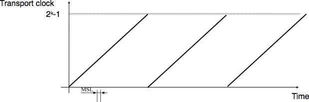
A classical solution to avoid remembering the previous transport connections to detect duplicates is to use a clock inside each transport entity. This transport clock has the following characteristics :
- the transport clock is implemented as a k bits counter and its clock cycle is such that 2k × cycle >> MSL. Furthermore, the transport clock counter is incremented every clock cycle and after each connection establishment. This clock is illustrated in the figure below.
- the transport clock must continue to be incremented even if the transport entity stops or reboots
It should be noted that transport clocks do not need and usually are not synchronised to the real-time clock. Precisely synchronising real-time clocks is an interesting problem, but it is outside the scope of this document. See [Mills2006] for a detailed discussion on synchronising the real-time clock.
The transport clock is combined with an exchange of three segments, called the three way handshake, to detect duplicates. This three way handshake occurs as follows:
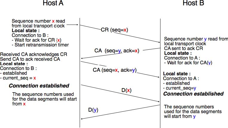
- The initiating transport entity sends a CR segment. This segment requests the establishment of a transport connection. It contains a connection identifier (not shown in the figure) and a sequence number (seq=x in the figure below) whose value is extracted from the transport clock . The transmission of the CR segment is protected by a retransmission timer.
- The remote transport entity processes the CR segment and creates state for the connection attempt. At this stage, the remote entity does not yet know whether this is a new connection attempt or a duplicate segment. It returns a CA segment that contains an acknowledgement number to confirm the reception of the CR segment (ack=x in the figure below) and a sequence number (seq=y in the figure below) whose value is extracted from its transport clock. At this stage, the connection is not yet established.
- The initiating entity receives the CA segment. The acknowledgement number of this segment confirms that the remote entity has correctly received the CA segment. The transport connection is considered to be established by the initiating entity and the numbering of the data segments starts at sequence number x. Before sending data segments, the initiating entity must acknowledge the received CA segments by sending another CA segment.
- The remote entity considers the transport connection to be established after having received the segment that acknowledges its CA segment. The numbering of the data segments sent by the remote entity starts at sequence number y.
The three way handshake is illustrated in the figure below.
Thanks to the three way handshake, transport entities avoid duplicate transport connections. This is illustrated by the three scenarios below.
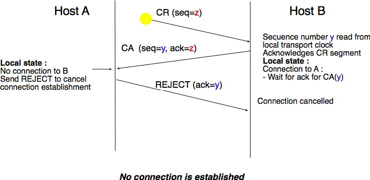
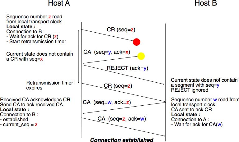
The first scenario is when the remote entity receives an old CR segment. It considers this CR segment as a connection establishment attempt and replies by sending a CA segment. However, the initiating host cannot match the received CA segment with a previous connection attempt. It sends a control segment (REJECT in the figure below) to cancel the spurious connection attempt. The remote entity cancels the connection attempt upon reception of this control segment.
A second scenario is when the initiating entity sends a CR segment that does not reach the remote entity and receives a duplicate CA segment from a previous connection attempt. This duplicate CA segment cannot contain a valid acknowledgement for the CR segment as the sequence number of the CR segment was extracted from the transport clock of the initiating entity. The CA segment is thus rejected and the CR segment is retransmitted upon expiration of the retransmission timer.
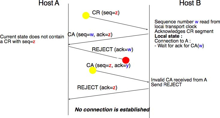
The last scenario is less likely, but it it important to consider it as well. The remote entity receives an old CR segment. It notes the connection attempt and acknowledges it by sending a CA segment. The initiating entity does not have a matching connection attempt and replies by sending a REJECT. Unfortunately, this segment never reaches the remote entity. Instead, the remote entity receives a retransmission of an older CA segment that contains the same sequence number as the first CR segment. This CA segment cannot be accepted by the remote entity as a confirmation of the transport connection as its acknowledgement number cannot have the same value as the sequence number of the first CA segment.
When we discussed the connection-oriented service, we mentioned that there are two types of connection releases : abrupt release and graceful release.
The first solution to release a transport connection is to define a new control segment (e.g. the DR segment) and consider the connection to be released once this segment has been sent or received. This is illustrated in the figure below.
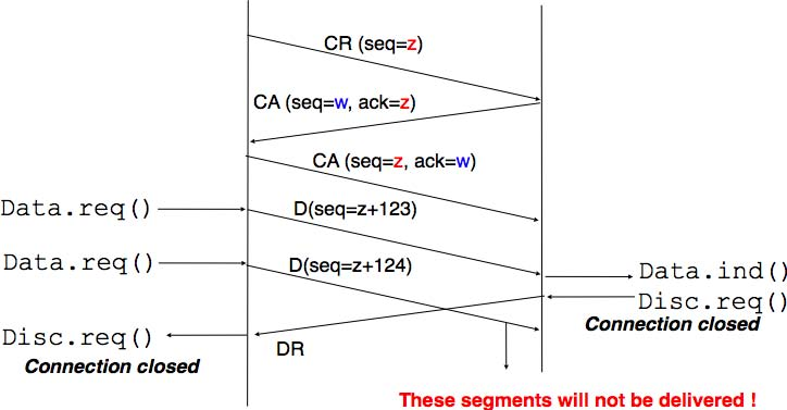
As the entity that sends the DR segment cannot know whether the other entity has already sent all its data on the connection, SDUs can be lost during such an abrupt connection release.
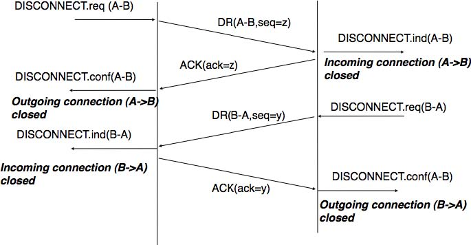
The second method to release a transport connection is to release independently the two directions of data transfer. Once a user of the transport service has sent all its SDUs, it performs a DISCONNECT.req for its direction of data transfer. The transport entity sends a control segment to request the release of the connection after the delivery of all previous SDUs to the remote user. This is usually done by placing in the DR the next sequence number and by delivering the DISCONNECT.ind only after all previous DATA.ind. The remote entity confirms the reception of the DR segment and the release of the corresponding direction of data transfer by returning an acknowledgement. This is illustrated in the figure below.
- 4223 reads
