


For most of the work you do in this book, you will use a histogram to display the data. One advantage of a histogram is that it can readily display large data sets. A rule of thumb is to use a histogram when the data set consists of 100 values or more.
A histogram consists of contiguous boxes. It has both a horizontal axis and a vertical axis. The horizontal axis is labeled with what the data represents (for instance, distance from your home to school). The vertical axis is labeled either Frequency or relative frequency. The graph will have the same shape with either label. The histogram (like the stemplot) can give you the shape of the data, the center, and the spread of the data. (The next section tells you how to calculate the center and the spread.)
The relative frequency is equal to the frequency for an observed value of the data divided by the total number of data values in the sample. (In the chapter on Sampling and Data (Section 1.1), we defined frequency as the number of times an answer occurs.) If:
- f = frequency
- n = total number of data values (or the sum of the individual frequencies), and
- RF = relative frequency,
then:

For example, if 3 students in Mr. Ahab's English class of 40 students received from 90% to 100%, then,
Seven and a half percent of the students received 90% to 100%. Ninety percent to 100% are quantitative measures.
To construct a histogram, first decide how many bars or intervals, also called classes, represent the data. Many histograms consist of from 5 to 15 bars or classes for clarity. Choose a starting point for the first interval to be less than the smallest data value. A convenient starting point is a lower value carried out to one more decimal place than the value with the most decimal places. For example, if the value with the most decimal places is 6.1 and this is the smallest value, a convenient starting point is 6.05 (6.1 - 0.05 = 6.05). We say that 6.05 has more precision. If the value with the most decimal places is 2.23 and the lowest value is 1.5, a convenient starting point is 1.495 (1.5 - 0.005 = 1.495). If the value with the most decimal places is 3.234 and the lowest value is 1.0, a convenient starting point is 0.9995 (1.0 - .0005 = 0.9995). If all the data happen to be integers and the smallest value is 2, then a convenient starting point is 1.5 (2 - 0.5 = 1.5). Also, when the starting point and other boundaries are carried to one additional decimal place, no data value will fall on a boundary.
Example 2.1
The following data are the heights (in inches to the nearest half inch) of 100 male semiprofessional soccer players. The heights are continuous data since height
is measured.
60; 60.5; 61; 61; 61.5
63.5; 63.5; 63.5
64; 64; 64; 64; 64; 64; 64; 64.5; 64.5; 64.5; 64.5; 64.5; 64.5; 64.5; 64.5
66; 66; 66; 66; 66; 66; 66; 66; 66; 66; 66.5; 66.5; 66.5; 66.5; 66.5; 66.5; 66.5; 66.5; 66.5; 66.5; 66.5;
67; 67; 67; 67; 67; 67; 67; 67; 67; 67; 67; 67; 67.5; 67.5; 67.5; 67.5; 67.5; 67.5; 67.5
68; 68; 69; 69; 69; 69; 69; 69; 69; 69; 69; 69; 69.5; 69.5; 69.5; 69.5; 69.5
70; 70; 70; 70; 70; 70; 70.5; 70.5; 70.5; 71; 71; 71
72; 72; 72; 72.5; 72.5; 73; 73.5
74
The smallest data value is 60. Since the data with the most decimal places has one decimal (for instance, 61.5), we want our starting point to have two decimal places. Since the numbers 0.5,
0.05, 0.005, etc. are convenient numbers, use 0.05 and subtract it from 60, the smallest value, for the convenient starting point.
60 - 0.05 = 59.95 which is more precise than, say, 61.5 by one decimal place. The starting point is, then, 59.95.
The largest value is 74. 74 + 0.05 = 74.05 is the ending value.
Next, calculate the width of each bar or class interval. To calculate this width, subtract the starting point from the ending value and divide by the number of bars (you must choose the
number of bars you desire). Suppose you choose 8 bars.
The boundaries are:
- 59.95
- 59.95 + 2 = 61.95
- 61.95 + 2 = 63.95
- 63.95 + 2 = 65.95
- 65.95 + 2 = 67.95
- 67.95 + 2 = 69.95
- 69.95 + 2 = 71.95
- 71.95 + 2 = 73.95
- 73.95 + 2 = 75.95
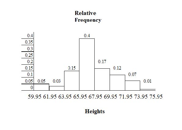
The heights 60 through 61.5 inches are in the interval 59.95 - 61.95. The heights that are 63.5 are in the interval 61.95 - 63.95. The heights that are 64 through 64.5 are in the interval
63.95 - 65.95. The heights 66 through 67.5 are in the interval 65.95 - 67.95. The heights 68 through 69.5 are in the interval 67.95 - 69.95. The heights 70 through 71 are in the interval
69.95 - 71.95. The heights 72 through 73.5 are in the interval 71.95 - 73.95. The height 74 is in the interval 73.95 - 75.95.
The following histogram displays the heights on the x-axis and relative frequency on the y-axis.
Example 2.2
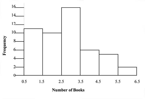
The following data are the number of books bought by 50 part-time college students at ABC College. The number of books is discrete data since books are counted.
1; 1; 1; 1; 1; 1; 1; 1; 1; 1; 1
2; 2; 2; 2; 2; 2; 2; 2; 2; 2
3; 3; 3; 3; 3; 3; 3; 3; 3; 3; 3; 3; 3; 3; 3; 3
4; 4; 4; 4; 4; 4
5; 5; 5; 5; 5
6; 6
Eleven students buy 1 book. Ten students buy 2 books. Sixteen students buy 3 books. Six students buy 4 books. Five students buy 5 books. Two students buy 6 books.
Because the data are integers, subtract 0.5 from 1, the smallest data value and add 0.5 to 6, the largest data value. Then the starting point is 0.5 and the ending value is 6.5.
Problem
Next, calculate the width of each bar or class interval. If the data are discrete and there are not too many different values, a width that places the data values in the middle of the bar or
class interval is the most convenient. Since the data consist of the numbers 1, 2, 3, 4, 5, 6 and the starting point is 0.5, a width of one places the 1 in the middle of the interval from 0.5
to 1.5, the 2 in the middle of the interval from 1.5 to 2.5, the 3 in the middle of the interval from 2.5 to 3.5, the 4 in the middle of the interval from ______ to ______, the 5 in the
middle of the interval from to ______, and the ______in the middle of the interval from ______to ______ .
Calculate the number of bars as follows:
where 1 is the width of a bar. Therefore, bars = 6.
The following histogram displays the number of books on the x-axis and the frequency on the y-axis.
Using the TI-83, 83+, 84, 84+ Calculator Instructions
Go to the Appendix (14:Appendix) in the menu on the left. There are calculator instructions for entering data and for creating a customized histogram. Create the histogram for Example 2.
- Press Y=. Press CLEAR to clear out any equations.
- Press STAT 1:EDIT. If L1 has data in it, arrow up into the name L1, press CLEAR and arrow down. If necessary, do the same for L2.
- Into L1, enter 1, 2, 3, 4, 5, 6
- Into L2, enter 11, 10, 16, 6, 5, 2
- Press WINDOW. Make Xmin = .5, Xmax = 6.5, Xscl = (6.5 -.5)/6, Ymin = -1, Ymax = 20, Yscl = 1, Xres = 1
- Press 2nd Y =. Start by pressing 4:Plotsof ENTER.
- Press 2nd Y =. Press 1:Plot1. Press ENTER. Arrow down to TYPE. Arrow to the 3rd picture (histogram). Press ENTER.
- Arrow down to Xlist: Enter L1 (2nd 1). Arrow down to Freq. Enter L2 (2nd 2).
- Press GRAPH
- Use the TRACE key and the arrow keys to examine the histogram.
- 瀏覽次數:3661
