


An important characteristic of any set of data is the variation in the data. In some data sets, the data values are concentrated closely near the mean; in other data sets, the data values are more widely spread out from the mean. The most common measure of variation, or spread, is the standard deviation.
The standard deviation is a number that measures how far data values are from their mean. The standard deviation
- provides a numerical measure of the overall amount of variation in a data set
- can be used to determine whether a particular data value is close to or far from the mean
The standard deviation provides a measure of the overall variation in a data set
The standard deviation is always positive or 0. The standard deviation is small when the data are all concentrated close to the mean, exhibiting little variation or spread. The standard deviation is larger when the data values are more spread out from the mean, exhibiting more variation.
Suppose that we are studying waiting times at the checkout line for customers at supermarket A and supermarket B; the average wait time at both markets is 5 minutes. At market A, the standard deviation for the waiting time is 2 minutes; at market B the standard deviation for the waiting time is 4 minutes.
Because market B has a higher standard deviation, we know that there is more variation in the waiting times at market B. Overall, wait times at market B are more spread out from the average; wait times at market A are more concentrated near the average.
The standard deviation can be used to determine whether a data value is close to or far from the mean.
Suppose that Rosa and Binh both shop at Market A. Rosa waits for 7 minutes and Binh waits for 1 minute at the checkout counter. At market A, the mean wait time is 5 minutes and the standard deviation is 2 minutes. The standard deviation can be used to determine whether a data value is close to or far from the mean.
Rosa waits for 7 minutes:
- 7 is 2 minutes longer than the average of 5; 2 minutes is equal to one standard deviation.
- Rosa's wait time of 7 minutes is 2 minutes longer than the average of 5 minutes.
- Rosa's wait time of 7 minutes is one standard deviation above the average of 5 minutes.
Binh waits for 1 minute.
- 1 is 4 minutes less than the average of 5; 4 minutes is equal to two standard deviations.
- Binh's wait time of 1 minute is 4 minutes less than the average of 5 minutes.
- Binh's wait time of 1 minute is two standard deviations below the average of 5 minutes.
- A data value that is two standard deviations from the average is just on the borderline for what many statisticians would consider to be far from the average. Considering data to be far from the mean if it is more than 2 standard deviations away is more of an approximate "rule of thumb" than a rigid rule. In general, the shape of the distribution of the data afects how much of the data is further away than 2 standard deviations. (We will learn more about this in later chapters.)
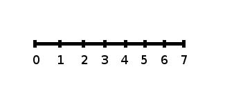
The number line may help you understand standard deviation. If we were to put 5 and 7 on a number line, 7 is to the right of 5. We say, then, that 7 is one standard deviation to the right of 5 because 5 + (1)(2) = 7.
If 1 were also part of the data set, then 1 is two standard deviations to the left of 5 because 5 + (−2)(2) = 1.
- In general, a value = mean + (#ofSTDEV)(standard deviation)
- where #ofSTDEVs = the number of standard deviations
- 7 is one standard deviation more than the mean of 5 because: 7 = 5 + (1)(2)
- 1 is two standard deviations less than the mean of 5 because: 1 = 5 + (−2)(2)
The equation value = mean + (#ofSTDEVs)(standard deviation) can be expressed for a sample and for a population:
-
sample:

-
Population:

The lower case letter s represents the sample standard deviation and the Greek letter σ (sigma, lower case) represents the population standard deviation.
The symbol  is the sample mean and the Greek symbol µ is the
population mean.
is the sample mean and the Greek symbol µ is the
population mean.
Calculating the Standard Deviation
If x is a number, then the diference "x - mean" is called its deviation. In a data set, there are as many deviations as there are items in the data set. The deviations are used
to calculate the standard deviation. If the numbers belong to a population, in symbols a deviation is x − µ . For sample data, in symbols a deviation is  .
.
The procedure to calculate the standard deviation depends on whether the numbers are the entire population or are data from a sample. The calculations are similar, but not identical. Therefore the symbol used to represent the standard deviation depends on whether it is calculated from a population or a sample. The lower case letter s represents the sample standard deviation and the Greek letter σ (sigma, lower case) represents the population standard deviation. If the sample has the same characteristics as the population, then s should be a good estimate of σ.
 values for a sample, or the x − µ values for a population). The
symbol σ2 represents the population variance; the population standard deviation σ is the square root of the population variance. The symbol s2 represents the sample
variance; the sample standard deviation s is the square root of the sample variance. You can think of the standard deviation as a special average of the deviations.
values for a sample, or the x − µ values for a population). The
symbol σ2 represents the population variance; the population standard deviation σ is the square root of the population variance. The symbol s2 represents the sample
variance; the sample standard deviation s is the square root of the sample variance. You can think of the standard deviation as a special average of the deviations.
If the numbers come from a census of the entire population and not a sample, when we calculate the average of the squared deviations to find the variance, we divide by N, the number of items in the population. If the data are from a sample rather than a population, when we calculate the average of the squared deviations, we divide by n-1, one less than the number of items in the sample. You can see that in the formulas below.
Formulas for the Sample Standard Deviation
-
 or
or 
- For the sample standard deviation, the denominator is n-1, that is the sample size MINUS 1.
Formulas for the Population Standard Deviation
-
 or
or 
- For the population standard deviation, the denominator is N, the number of items in the population.
In these formulas, f represents the frequency with which a value appears. For example, if a value appears once, f is 1. If a value appears three times in the data set or population, f is 3.
Sampling Variability of a Statistic
The statistic of a sampling distribution was discussed in Descriptive Statistics: Measuring the Center of the Data. How much the statistic varies from one sample
to another is known as the sampling variability of a statistic. You typically measure the sampling variability of a statistic by its
standard error. The standard error of the mean is an example of a standard error. It is a special standard deviation and is known as the standard deviation of the
sampling distribution of the mean. You will cover the standard error of the mean in The Central Limit Theorem (not now). The notation for the standard error of the
mean is  where σ is the standard deviation of the
population and n is the size of the sample.
where σ is the standard deviation of the
population and n is the size of the sample.
Example 2.7
In a fifth grade class, the teacher was interested in the average age and the sample standard deviation of the ages of her students. The following data are the ages for a SAMPLE of n = 20
fifth grade students. The ages are rounded to the nearest half year:
9 ; 9.5 ; 9.5 ; 10 ; 10 ; 10 ; 10 ; 10.5 ; 10.5 ; 10.5 ; 10.5 ; 11 ; 11 ; 11 ; 11 ; 11 ; 11 ; 11.5 ; 11.5 ; 11.5

The average age is 10.53 years, rounded to 2 places.
The variance may be calculated by using a table. Then the standard deviation is calculated by taking the square root of the variance. We will explain the parts of the table after
calculatings.
|
Data |
Freq. |
Deviations |
Deviations2 |
(Freq.)(Deviations2) |
|---|---|---|---|---|
|
x |
f |
|
|
|
|
9 |
1 |
9 − 10.525 = −1.525 |
(−1.525)2 = 2.325625 |
1 × 2.325625 = 2.325625 |
|
9.5 |
2 |
9.5 − 10.525 = −1.025 |
(−1.025)2 = 1.050625 |
2 × 1.050625 = 2.101250 |
|
10 |
4 |
10 − 10.525 = −0.525 |
(−0.525)2 = 0.275625 |
4 × .275625 = 1.1025 |
|
10.5 |
4 |
10.5 − 10.525 = −0.025 |
(−0.025)2 = 0.000625 |
4 × .000625 = .0025 |
|
11 |
6 |
11 − 10.525 = 0.475 |
(0.475)2 = 0.225625 |
6 × .225625 = 1.35375 |
|
11.5 |
3 |
11.5 − 10.525 = 0.975 |
(0.975)2 = 0.950625 |
3 × .950625 = 2.851875 |


The sample variance, s2, is equal to the sum of the last column (9.7375) divided by the total number of data values minus one (20 - 1):
The sample standard deviation s is equal to the square root of the sample variance:
Rounded to two decimal places, s =0.72
Typically, you do the calculation for the standard deviation on your calculator or computer. The intermediate results are not
rounded. This is done for accuracy.
Problem 1
Verify the mean and standard deviation calculated above on your calculator or computer.
Solution
Using the TI-83,83+,84+ Calculators
- Enter data into the list editor. Press STAT 1:EDIT. If necessary, clear the lists by arrowing up into the name. Press CLEAR and arrow down.
- Put the data values (9, 9.5, 10, 10.5, 11, 11.5) into list L1 and the frequencies (1, 2, 4, 4, 6, 3) into list L2. Use the arrow keys to move around.
- Press STAT and arrow to CALC. Press 1:1-VarStats and enter L1 (2nd 1), L2 (2nd 2). Do not forget the comma. Press ENTER.
-

- Use Sx because this is sample data (not a population): Sx = 0.715891
- For the following problems, recall that value = mean + (#ofSTDEVs)(standard deviation)
- For a sample:

- For a population:

- For this example, use
 because the data is
from a sample
because the data is
from a sample
Problem 2
Find the value that is 1 standard deviation above the mean. Find 
Solution

Problem 3
Find the value that is two standard deviations below the mean. Find 
Solution

Problem 4
Find the values that are 1.5 standard deviations from (below and above) the mean.
Solution
Explanation of the standard deviation calculation shown in the table
The deviations show how spread out the data are about the mean. The data value 11.5 is farther from the mean than is the data value 11. The deviations 0.97 and 0.47 indicate that. A positive deviation occurs when the data value is greater than the mean. A negative deviation occurs when the data value is less than the mean; the deviation is -1.525 for the data value 9. If you add the deviations, the sum is always zero. (For this example, there are n=20 deviations.) So you cannot simply add the deviations to get the spread of the data. By squaring the deviations, you make them positive numbers, and the sum will also be positive. The variance, then, is the average squared deviation.
The variance is a squared measure and does not have the same units as the data. Taking the square root solves the problem. The standard deviation measures the spread in the same units as the data.
Notice that instead of dividing by n=20, the calculation divided by n-1=20-1=19 because the data is a sample. For the sample variance, we divide by the sample size minus one (n − 1). Why not divide by n? The answer has to do with the population variance. The sample variance is an estimate of the population variance. Based on the theoretical mathematics that lies behind these calculations, dividing by (n − 1) gives a better estimate of the population variance.
The standard deviation, s or σ, is either zero or larger than zero. When the standard deviation is 0, there is no spread; that is, the all the data values are equal to each other. The standard deviation is small when the data are all concentrated close to the mean, and is larger when the data values show more variation from the mean. When the standard deviation is a lot larger than zero, the data values are very spread out about the mean; outliers can make s or σ very large.
The standard deviation, when first presented, can seem unclear. By graphing your data, you can get a better "feel" for the deviations and the standard deviation. You will find that in symmetrical distributions, the standard deviation can be very helpful but in skewed distributions, the standard deviation may not be much help. The reason is that the two sides of a skewed distribution have different spreads. In a skewed distribution, it is better to look at the first quartile, the median, the third quartile, the smallest value, and the largest value. Because numbers can be confusing, always graph your data.
Example 2.8
Use the following data (first exam scores) from Susan Dean's spring pre-calculus class:
33; 42; 49; 49; 53; 55; 55; 61; 63; 67; 68; 68; 69; 69; 72; 73; 74; 78; 80; 83; 88; 88; 88; 90; 92; 94; 94; 94; 94; 96; 100
- Create a chart containing the data, frequencies, relative frequencies, and cumulative relative frequencies to three decimal places.
- Calculate the following to one decimal place using a TI-83+ or TI-84 calculator:
- The sample mean
- The sample standard deviation
- The median
- The first quartile
- The third quartile
- IQR
- Construct a box plot and a histogram on the same set of axes. Make comments about the box plot, the histogram, and the chart.
Solution
-
Data
Frequency
Relative Frequency
Cumulative Relative Frequency
33
1
0.032
0.032
42
1
0.032
0.064
49
2
0.065
0.129
53
1
0.032
0.161
55
2
0.065
0.226
61
1
0.032
0.258
63
1
0.032
0.29
67
1
0.032
0.322
68
2
0.065
0.387
69
2
0.065
0.452
72
1
0.032
0.484
73
1
0.032
0.516
74
1
0.032
0.548
78
1
0.032
0.580
80
1
0.032
0.612
83
1
0.032
0.644
88
3
0.097
0.741
90
1
0.032
0.773
92
1
0.032
0.805
94
4
0.129
0.934
96
1
0.032
0.966
100
1
0.032
0.998 (Why isn't this value 1?)
-
- The sample mean = 73.5
- The sample standard deviation = 17.9
- The median = 73
- The first quartile = 61
- The third quartile = 90
- IQR = 90 - 61 = 29
- The x-axis goes from 32.5 to 100.5; y-axis goes from -2.4 to 15 for the histogram; number of intervals is 5 for the histogram so the width of an interval is (100.5 -32.5) divided by 5 which is equal to 13.6. Endpoints of the intervals: starting point is 32.5, 32.5+13.6 = 46.1, 46.1+13.6 = 59.7, 59.7+13.6 = 73.3, 73.3+13.6 = 86.9, 86.9+13.6 = 100.5 the ending value; No data values fall on an interval boundary.
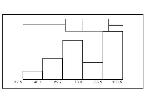
The long left whisker in the box plot is refected in the left side of the histogram. The spread of the exam scores in the lower 50% is greater (73 - 33 = 40) than the spread in the upper 50% (100 - 73 = 27). The histogram, box plot, and chart all refect this. There are a substantial number of A and B grades (80s, 90s, and 100). The histogram clearly shows this. The box plot shows us that the middle 50% of the exam scores (IQR = 29) are Ds, Cs, and Bs. The box plot also shows us that the lower 25% of the exam scores are Ds and Fs.
Comparing Values from Different Data Sets
The standard deviation is useful when comparing data values that come from different data sets. If the data sets have different means and standard deviations, it can be misleading to compare the data values directly.
- For each data value, calculate how many standard deviations the value is away from its mean.
- Use the formula: value = mean + (#ofSTDEVs)(standard deviation); solve for #ofSTDEVs.
- Compare the results of this calculation.
#ofSTDEVs is often called a "z-score"; we can use the symbol z. In symbols, the formulas become:
| Sample |

|

|
| Population |

|

|
Example 2.9
Two students, John and Ali, from different high schools, wanted to find out who had the highest G.P.A. when compared to his school. Which student had the highest G.P.A. when compared to his school?
|
Student |
GPA |
School Mean GPA |
School Standard Deviation |
|---|---|---|---|
|
John |
2.85 |
3.0 |
0.7 |
|
Ali |
77 |
80 |
10 |
For each student, determine how many standard deviations (#ofSTDEVs) his GPA is away from the average, for his school. Pay careful attention to signs when comparing and interpreting the
answer.
John has the better G.P.A. when compared to his school because his G.P.A. is 0.21 standard deviations below his school's mean while Ali's G.P.A. is 0.3 standard
deviations below his school's mean.
John's z-score of −0.21 is higher than Ali's z-score of −0.3 . For GPA, higher values are better, so we conclude that John has the better GPA when compared to his school.
The following lists give a few facts that provide a little more insight into what the standard deviation tells us about the distribution of the data.
For ANY data set, no matter what the distribution of the data is:
- At least 75% of the data is within 2 standard deviations of the mean.
- At least 89% of the data is within 3 standard deviations of the mean.
- At least 95% of the data is within 4 1/2 standard deviations of the mean.
- This is known as Chebyshev's Rule.
For data having a distribution that is MOUND-SHAPED and SYMMETRIC:
- Approximately 68% of the data is within 1 standard deviation of the mean.
- Approximately 95% of the data is within 2 standard deviations of the mean.
- More than 99% of the data is within 3 standard deviations of the mean.
- This is known as the Empirical Rule.
- It is important to note that this rule only applies when the shape of the distribution of the data is mound-shaped and symmetric. We will learn more about this when studying the "Normal" or "Gaussian" probability distribution in later chapters.
**With contributions from Roberta Bloom
- 瀏覽次數:5651
