


Next we illustrate the relationship between Acme’s total product curve and its total costs. Acme can vary the quantity of labor it uses each day, so the cost of this labor is a variable cost. We assume capital is a fixed factor of production in the short run, so its cost is a fixed cost.
Suppose that Acme pays a wage of $100 per worker per day. If labor is the only variable factor, Acme’s total variable costs per day amount to $100 times the number of workers it employs. We can use the information given by the total product curve, together with the wage, to compute Acme’s total variable costs.
We know from Figure 8.1 that Acme requires 1 worker working 1 day to produce 1 jacket. The total variable cost of a jacket thus equals $100. Three units of labor produce 7 jackets per day; the total variable cost of 7 jackets equals $300. Figure 8.4 shows Acme’s total variable costs for producing each of the output levels given in Figure 8.1"
Figure 8.4 gives us costs for several quantities of jackets, but we need a bit more detail. We know, for example, that 7 jackets have a total variable cost of $300. What is the total variable cost of 6 jackets?
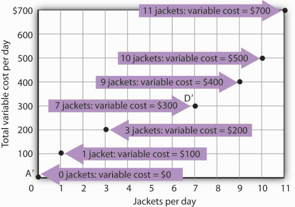
The points shown give the variable costs of producing the quantities of jackets given in the total product curve in Figure 8.1 and Figure 8.2. Suppose Acme’s workers earn $100 per day. If Acme produces 0 jackets, it will use no labor—its variable cost thus equals $0 (Point A′). Producing 7 jackets requires 3 units of labor; Acme’s variable cost equals $300 (Point D′).
We can estimate total variable costs for other quantities of jackets by inspecting the total product curve in Figure 8.1. Reading over from a quantity of 6 jackets to the total product curve and then down suggests that the Acme needs about 2.8 units of labor to produce 6 jackets per day. Acme needs 2 full-time and 1 part-time tailors to produce 6 jackets. Figure 8.5 gives the precise total variable costs for quantities of jackets ranging from 0 to 11 per day. The numbers in boldface type are taken from Figure 8.4; the other numbers are estimates we have assigned to produce a total variable cost curve that is consistent with our total product curve. You should, however, be certain that you understand how the numbers in boldface type were found.
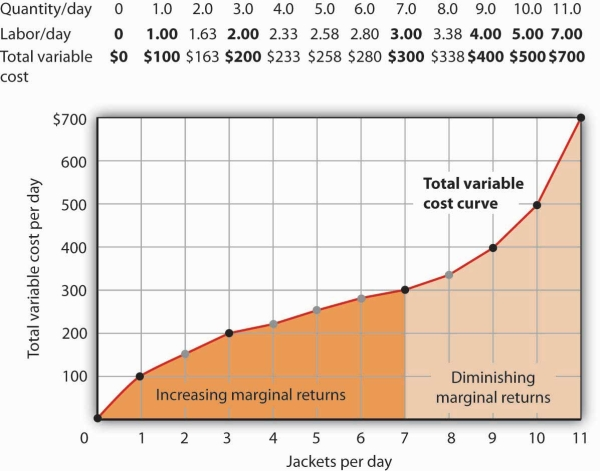
Total variable costs for output levels shown in Acme’s total product curve were shown in Figure 8.4. To complete the total variable cost curve, we need to know the variable cost for each level of output from 0 to 11 jackets per day. The variable costs and quantities of labor given in Figure 8.4 are shown in boldface in the table here and with black dots in the graph. The remaining values were estimated from the total product curve in Figure 8.1 and Figure 8.2. For example, producing 6 jackets requires 2.8 workers, for a variable cost of $280.
Suppose Acme’s present plant, including the building and equipment, is the equivalent of 20 units of capital. Acme has signed a long-term lease for these 20 units of capital at a cost of $200 per day. In the short run, Acme cannot increase or decrease its quantity of capital—it must pay the $200 per day no matter what it does. Even if the firm cuts production to zero, it must still pay $200 per day in the short run.
Acme’s total cost is its total fixed cost of $200 plus its total variable cost. We add $200 to the total variable cost curve in Figure 8.5 to get the total cost curve shown in Figure 8.6.
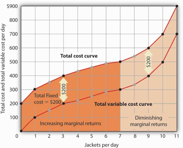
We add total fixed cost to the total variable cost to obtain total cost. In this case, Acme’s total fixed cost equals $200 per day.
Notice something important about the shapes of the total cost and total variable cost curves in Figure 8.6. The total cost curve, for example, starts at $200 when Acme produces 0 jackets—that is its total fixed cost. The curve rises, but at a decreasing rate, up to the seventh jacket. Beyond the seventh jacket, the curve becomes steeper and steeper. The slope of the total variable cost curve behaves in precisely the same way.
Recall that Acme experienced increasing marginal returns to labor for the first three units of labor—or the first seven jackets. Up to the third worker, each additional worker added more and more to Acme’s output. Over the range of increasing marginal returns, each additional jacket requires less and less additional labor. The first jacket required one tailor; the second required the addition of only a part-time tailor; the third required only that Acme boost that part-time tailor’s hours to a full day. Up to the seventh jacket, each additional jacket requires less and less additional labor, and thus costs rise at a decreasing rate; the total cost and total variable cost curves become flatter over the range of increasing marginal returns.
Acme experiences diminishing marginal returns beyond the third unit of labor—or the seventh jacket. Notice that the total cost and total variable cost curves become steeper and steeper beyond this level of output. In the range of diminishing marginal returns, each additional unit of a factor adds less and less to total output. That means each additional unit of output requires larger and larger increases in the variable factor, and larger and larger increases in costs.
- 2700 reads
