Adding the first worker increases Acme’s output from 0 to 1 jacket per day. The second tailor adds 2 jackets to total output; the third adds 4. The marginal product goes up because when there are more workers, each one can specialize to a degree. One worker might cut the cloth, another might sew the seams, and another might sew the buttonholes. Their increasing marginal products are reflected by the increasing slope of the total product curve over the first 3 units of labor and by the upward slope of the marginal product curve over the same range. The range over which marginal products are increasing is called the range of increasing marginal returns. Increasing marginal returns exist in the context of a total product curve for labor, so we are holding the quantities of other factors constant. Increasing marginal returns may occur for any variable factor.
The fourth worker adds less to total output than the third; the marginal product of the fourth worker is 2 jackets. The data in Figure 8.2 show that marginal product continues to decline after the fourth worker as more and more workers are hired. The additional workers allow even greater opportunities for specialization, but because they are operating with a fixed amount of capital, each new worker adds less to total output. The fifth tailor adds only a single jacket to total output. When each additional unit of a variable factor adds less to total output, the firm is experiencing diminishing marginal returns. Over the range of diminishing marginal returns, the marginal product of the variable factor is positive but falling. Once again, we assume that the quantities of all other factors of production are fixed. Diminishing marginal returns may occur for any variable factor. Panel (b) shows that Acme experiences diminishing marginal returns between the third and seventh workers, or between 7 and 11 jackets per day.
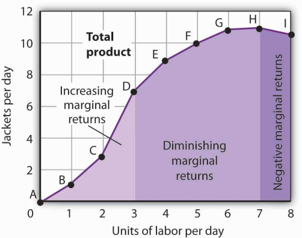
After the seventh unit of labor, Acme’s fixed plant becomes so crowded that adding another worker actually reduces output. When additional units of a variable factor reduce total output, given constant quantities of all other factors, the company experiences negative marginal returns. Now the total product curve is downward sloping, and the marginal product curve falls below zero. Figure 8.3 shows the ranges of increasing, diminishing, and negative marginal returns. Clearly, a firm will never intentionally add so much of a variable factor of production that it enters a range of negative marginal returns.

This graph shows Acme’s total product curve from Figure 8.1 with the ranges of increasing marginal returns, diminishing marginal returns, and negative marginal returns marked. Acme experiences increasing marginal returns between 0 and 3 units of labor per day, diminishing marginal returns between 3 and 7 units of labor per day, and negative marginal returns beyond the 7th unit of labor.
The idea that the marginal product of a variable factor declines over some range is important enough, and general enough, that economists state it as a law. The law of diminishing marginal returns holds that the marginal product of any variable factor of production will eventually decline, assuming the quantities of other factors of production are unchanged.
Heads Up!
It is easy to confuse the concept of diminishing marginal returns with the idea of negative marginal returns. To say a firm is experiencing diminishing marginal returns is not to say its output is falling. Diminishing marginal returns mean that the marginal product of a variable factor is declining. Output is still increasing as the variable factor is increased, but it is increasing by smaller and smaller amounts. As we saw in Figure 8.2 and Figure 8.3, the range of diminishing marginal returns was between the third and seventh workers; over this range of workers, output rose from 7 to 11 jackets. Negative marginal returns started after the seventh worker.
To see the logic of the law of diminishing marginal returns, imagine a case in which it does not hold. Say that you have a small plot of land for a vegetable garden, 10 feet by 10 feet in size. The plot itself is a fixed factor in the production of vegetables. Suppose you are able to hold constant all other factors—water, sunshine, temperature, fertilizer, and seed—and vary the amount of labor devoted to the garden. How much food could the garden produce? Suppose the marginal product of labor kept increasing or was constant. Then you could grow an unlimited quantity of food on your small plot—enough to feed the entire world! You could add an unlimited number of workers to your plot and still increase output at a constant or increasing rate. If you did not get enough output with, say, 500 workers, you could use 5 million; the five-millionth worker would add at least as much to total output as the first. If diminishing marginal returns to labor did not occur, the total product curve would slope upward at a constant or increasing rate.
The shape of the total product curve and the shape of the resulting marginal product curve drawn in Figure 8.2 are typical of any firm for the short run. Given its fixed factors of production, increasing the use of a variable factor will generate increasing marginal returns at first; the total product curve for the variable factor becomes steeper and the marginal product rises. The opportunity to gain from increased specialization in the use of the variable factor accounts for this range of increasing marginal returns. Eventually, though, diminishing returns will set in. The total product curve will become flatter, and the marginal product curve will fall.
- 瀏覽次數:20017


