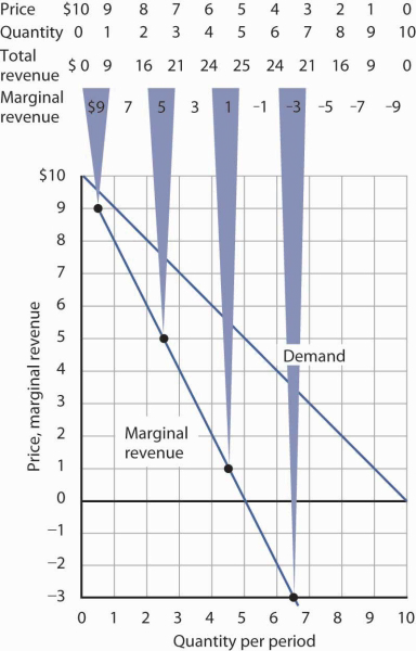
In the perfectly competitive case, the additional revenue a firm gains from selling an additional unit—its marginal revenue—is equal to the market price. The firm’s demand curve, which is a horizontal line at the market price, is also its marginal revenue curve. But a monopoly firm can sell an additional unit only by lowering the price. That fact complicates the relationship between the monopoly’s demand curve and its marginal revenue.
Suppose the firm in Figure 10.3Figure 10.4 sells 2 units at a price of $8 per unit. Its total revenue is $16. Now it wants to sell a third unit and wants to know the marginal revenue of that unit. To sell 3 units rather than 2, the firm must lower its price to $7 per unit. Total revenue rises to $21. The marginal revenue of the third unit is thus $5. But the price at which the firm sells 3 units is $7. Marginal revenue is less than price.
To see why the marginal revenue of the third unit is less than its price, we need to examine more carefully how the sale of that unit affects the firm’s revenues. The firm brings in $7 from the sale of the third unit. But selling the third unit required the firm to charge a price of $7 instead of the $8 the firm was charging for 2 units. Now the firm receives less for the first 2 units. The marginal revenue of the third unit is the $7 the firm receives for that unit minus the $1 reduction in revenue for each of the first two units. The marginal revenue of the third unit is thus $5. (In this chapter we assume that the monopoly firm sells all units of output at the same price. In the next chapter, we will look at cases in which firms charge different prices to different customers.)
Marginal revenue is less than price for the monopoly firm. Figure 10.4 shows the relationship between demand and marginal revenue, based on the demand curve introduced in Figure 10.3. As always, we follow the convention of plotting marginal values at the midpoints of the intervals.

The marginal revenue curve for the monopoly firm lies below its demand curve. It shows the additional revenue gained from selling an additional unit. Notice that, as always, marginal values are plotted at the midpoints of the respective intervals.
When the demand curve is linear, as in Figure 10.4, the marginal revenue curve can be placed according to the following rules: the marginal revenue curve is always below the demand curve and the marginal revenue curve will bisect any horizontal line drawn between the vertical axis and the demand curve. To put it another way, the marginal revenue curve will be twice as steep as the demand curve. The demand curve in Figure 10.4 is given by the equation Q=10−P, which can be written P=10−Q. The marginal revenue curve is given byP=10−2Q, which is twice as steep as the demand curve.
The marginal revenue and demand curves in Figure 10.4 follow these rules. The marginal revenue curve lies below the demand curve, and it bisects any horizontal line drawn from the vertical axis to the demand curve. At a price of $6, for example, the quantity demanded is 4. The marginal revenue curve passes through 2 units at this price. At a price of 0, the quantity demanded is 10; the marginal revenue curve passes through 5 units at this point.
Just as there is a relationship between the firm’s demand curve and the price elasticity of demand, there is a relationship between its marginal revenue curve and elasticity. Where marginal revenue is positive, demand is price elastic. Where marginal revenue is negative, demand is price inelastic. Where marginal revenue is zero, demand is unit price elastic.
|
When marginal revenue is … |
then demand is … |
|
positive, |
price elastic. |
|
negative, |
price inelastic. |
|
zero, |
unit price elastic. |
A firm would not produce an additional unit of output with negative marginal revenue. And, assuming that the production of an additional unit has some cost, a firm would not produce the extra unit if it has zero marginal revenue. Because a monopoly firm will generally operate where marginal revenue is positive, we see once again that it will operate in the elastic range of its demand curve.
- 瀏覽次數:2568


