To construct a combined production possibilities curve for all three plants, we can begin by asking how many pairs of skis Alpine Sports could produce if it were producing only skis. To find this quantity, we add up the values at the vertical intercepts of each of the production possibilities curves in Figure 2.3. These intercepts tell us the maximum number of pairs of skis each plant can produce. Plant 1 can produce 200 pairs of skis per month, Plant 2 can produce 100 pairs of skis at per month, and Plant 3 can produce 50 pairs. Alpine Sports can thus produce 350 pairs of skis per month if it devotes its resources exclusively to ski production. In that case, it produces no snowboards.
Now suppose the firm decides to produce 100 snowboards. That will require shifting one of its plants out of ski production. Which one will it choose to shift? The sensible thing for it to do is to choose the plant in which snowboards have the lowest opportunity cost—Plant 3. It has an advantage not because it can produce more snowboards than the other plants (all the plants in this example are capable of producing up to 100 snowboards per month) but because it is the least productive plant for making skis. Producing a snowboard in Plant 3 requires giving up just half a pair of skis.
Economists say that an economy has a comparative advantage in producing a good or service if the opportunity cost of producing that good or service is lower for that economy than for any other. Plant 3 has a comparative advantage in snowboard production because it is the plant for which the opportunity cost of additional snowboards is lowest. To put this in terms of the production possibilities curve, Plant 3 has a comparative advantage in snowboard production (the good on the horizontal axis) because its production possibilities curve is the flattest of the three curves.

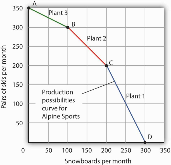
The curve shown combines the production possibilities curves for each plant. At point A, Alpine Sports produces 350 pairs of skis per month and no snowboards. If the firm wishes to increase snowboard production, it will first use Plant 3, which has a comparative advantage in snowboards.
Plant 3’s comparative advantage in snowboard production makes a crucial point about the nature of comparative advantage. It need not imply that a particular plant is especially good at an activity. In our example, all three plants are equally good at snowboard production. Plant 3, though, is the least efficient of the three in ski production. Alpine thus gives up fewer skis when it produces snowboards in Plant 3. Comparative advantage thus can stem from a lack of efficiency in the production of an alternative good rather than a special proficiency in the production of the first good.
The combined production possibilities curve for the firm’s three plants is shown in Figure 2.4. We begin at point A, with all three plants producing only skis. Production totals 350 pairs of skis per month and zero snowboards. If the firm were to produce 100 snowboards at Plant 3, ski production would fall by 50 pairs per month (recall that the opportunity cost per snowboard at Plant 3 is half a pair of skis). That would bring ski production to 300 pairs, at point B. If Alpine Sports were to produce still more snowboards in a single month, it would shift production to Plant 2, the facility with the next-lowest opportunity cost. Producing 100 snowboards at Plant 2 would leave Alpine Sports producing 200 snowboards and 200 pairs of skis per month, at point C. If the firm were to switch entirely to snowboard production, Plant 1 would be the last to switch because the cost of each snowboard there is 2 pairs of skis. With all three plants producing only snowboards, the firm is at point D on the combined production possibilities curve, producing 300 snowboards per month and no skis.
Notice that this production possibilities curve, which is made up of linear segments from each assembly plant, has a bowed-out shape; the absolute value of its slope increases as Alpine Sports produces more and more snowboards. This is a result of transferring resources from the production of one good to another according to comparative advantage. We shall examine the significance of the bowed-out shape of the curve in the next section.
- 瀏覽次數:2913


