We see in Figure 2.4 that, beginning at point A and producing only skis, Alpine Sports experiences higher and higher opportunity costs as it produces more snowboards. The fact that the opportunity cost of additional snowboards increases as the firm produces more of them is a reflection of an important economic law. The law of increasing opportunity cost holds that as an economy moves along its production possibilities curve in the direction of producing more of a particular good, the opportunity cost of additional units of that good will increase.
We have seen the law of increasing opportunity cost at work traveling from point A toward point D on the production possibilities curve in Figure 2.4. The opportunity cost of each of the first 100 snowboards equals half a pair of skis; each of the next 100 snowboards has an opportunity cost of 1 pair of skis, and each of the last 100 snowboards has an opportunity cost of 2 pairs of skis. The law also applies as the firm shifts from snowboards to skis. Suppose it begins at point D, producing 300 snowboards per month and no skis. It can shift to ski production at a relatively low cost at first. The opportunity cost of the first 200 pairs of skis is just 100 snowboards at Plant 1, a movement from point D to point C, or 0.5 snowboards per pair of skis. We would say that Plant 1 has a comparative advantage in ski production. The next 100 pairs of skis would be produced at Plant 2, where snowboard production would fall by 100 snowboards per month. The opportunity cost of skis at Plant 2 is 1 snowboard per pair of skis. Plant 3 would be the last plant converted to ski production. There, 50 pairs of skis could be produced per month at a cost of 100 snowboards, or an opportunity cost of 2 snowboards per pair of skis.
The bowed-out production possibilities curve for Alpine Sports illustrates the law of increasing opportunity cost. Scarcity implies that a production possibilities curve is downward sloping; the law of increasing opportunity cost implies that it will be bowed out, or concave, in shape.
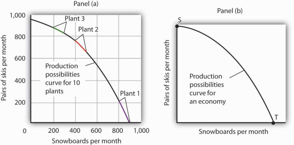
The bowed-out curve of Figure 2.4 becomes smoother as we include more production facilities. Suppose Alpine Sports expands to 10 plants, each with a linear production possibilities curve. Panel (a) of Figure 2.5 shows the combined curve for the expanded firm, constructed as we did in Figure 2.4. This production possibilities curve includes 10 linear segments and is almost a smooth curve. As we include more and more production units, the curve will become smoother and smoother. In an actual economy, with a tremendous number of firms and workers, it is easy to see that the production possibilities curve will be smooth. We will generally draw production possibilities curves for the economy as smooth, bowed-out curves, like the one in Panel (b). This production possibilities curve shows an economy that produces only skis and snowboards. Notice the curve still has a bowed-out shape; it still has a negative slope. Notice also that this curve has no numbers. Economists often use models such as the production possibilities model with graphs that show the general shapes of curves but that do not include specific numbers.

As we combine the production possibilities curves for more and more units, the curve becomes smoother. It retains its negative slope and bowed-out shape. In Panel (a) we have a combined production possibilities curve for Alpine Sports, assuming that it now has 10 plants producing skis and snowboards. Even though each of the plants has a linear curve, combining them according to comparative advantage, as we did with 3 plants in Figure 2.4, produces what appears to be a smooth, nonlinear curve, even though it is made up of linear segments. In drawing production possibilities curves for the economy, we shall generally assume they are smooth and “bowed out,” as in Panel (b). This curve depicts an entire economy that produces only skis and snowboards.
- 瀏覽次數:1868


