Suppose a college student, Laurie Phan, faces two midterms tomorrow, one in economics and another in accounting. She has already decided to spend 5 hours studying for the two examinations. This decision imposes a constraint on the problem. Suppose that Ms. Phan’s goal is to allocate her 5 hours of study so that she increases her total score for the two exams by as much as possible.
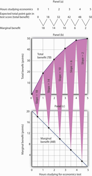
Ms. Phan expects the relationship between the time she spends studying for the economics exam and the total gain in her score to be as given by the second row of the table in Panel (a) of Figure 6.1. We interpret the expected total gain in her score as the total benefit of study. She expects that 1 hour of study will raise her score by 18 points; 2 hours will raise it by 32 points, and so on. These values are plotted in Panel (b). Notice that the total benefit curve rises, but by smaller and smaller amounts, as she studies more and more. The slope of the curve, which in this case tells us the rate at which her expected score rises with increased study time, falls as we travel up and to the right along the curve.

The table in Panel (a) shows the total benefit and marginal benefit of the time Laurie Phan spends studying for her economics exam. Panel (b) shows the total benefit curve. Panel (c) shows the marginal benefit curve, which is given by the slope of the total benefit curve in Panel (b).
Now look at the third row in the table in Panel (a). It tells us the amount by which each additional hour of study increases her expected score; it gives the marginal benefit of studying for the economics exam. Marginal benefit equals the amount by which total benefit rises with each additional hour of study. Because these marginal benefits are given by the changes in total benefits from additional hours of study, they equal the slope of the total benefit curve. We see this in the relationship between Panels (b) and (c) of Figure 6.1. The decreasing slope of the total benefit curve in Panel (b) gives us the downward-sloping marginal benefit curve in Panel (c).
The marginal benefit curve tells us what happens when we pass from one point to another on the total benefit curve, so we have plotted marginal benefits at the midpoints of the hourly intervals in Panel (c). For example, the total benefit curve in Panel (b) tells us that, when Ms. Phan increases her time studying for the economics exam from 2 hours to 3 hours, her total benefit rises from 32 points to 42 points. The increase of 10 points is the marginal benefit of increasing study time for the economics exam from 2 hours to 3 hours. We mark the point for a marginal benefit of 10 points midway between 2 and 3 hours. Because marginal values tell us what happens as we pass from one quantity to the next, we shall always plot them at the midpoints of intervals of the variable on the horizontal axis.
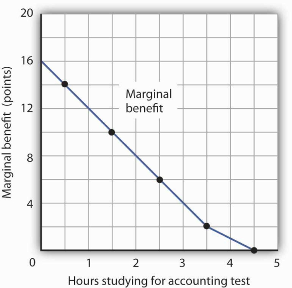
We can perform the same kind of analysis to obtain the marginal benefit curve for studying for the accounting exam. Figure 6.2 presents this curve. Like the marginal benefit curve for studying economics, it slopes downward. Once again, we have plotted marginal values at the midpoints of the intervals. Increasing study time in accounting from 0 to 1 hour increases Ms. Phan’s expected accounting score by 14 points.

The marginal benefit Laurie Phan expects from studying for her accounting exam is shown by the marginal benefit curve. The first hour of study increases her expected score by 14 points, the second hour by 10 points, the third by 6 points, and so on.
Ms. Phan’s marginal benefit curves for studying typify a general phenomenon in economics. Marginal benefit curves for virtually all activities, including the activities of consumers and of firms, slope downward. Think about your own experience with studying. On a given day, the first hour spent studying a certain subject probably generates a greater marginal benefit than the second, and the second hour probably generates a greater marginal benefit than the third. You may reach a point at which an extra hour of study is unlikely to yield any benefit at all. Of course, our example of Laurie Phan’s expected exam scores is a highly stylized one. One could hardly expect a student to have a precise set of numbers to guide him or her in allocating study time. But it is certainly the case that students have a rough idea of the likely payoff of study time in different subjects. If you were faced with exams in two subjects, it is likely that you would set aside a certain amount of study time, just as Ms. Phan did in our example. And it is likely that your own experience would serve as a guide in determining how to allocate that time. Economists do not assume that people have numerical scales in their heads with which to draw marginal benefit and marginal cost curves. They merely assume that people act as if they did.
The nature of marginal benefits can change with different applications. For a restaurant, the marginal benefit of serving one more meal can be defined as the revenue that meal produces. For a consumer, the marginal benefit of one more slice of pizza can be considered in terms of the additional satisfaction the pizza will create. But whatever the nature of the benefit, marginal benefits generally fall as quantities increase.
Ms. Phan’s falling marginal benefit from hours spent studying accounting has special significance for our analysis of her choice concerning how many hours to devote to economics. In our problem, she had decided to devote 5 hours to studying the two subjects. That means that the opportunity cost of an hour spent studying economics equals the benefit she would have gotten spending that hour studying accounting.
Suppose, for example, that she were to consider spending all 5 hours studying accounting. The marginal benefit curve for studying for her accounting exam tells us that she expects that the fifth hour will add nothing to her score. Shifting that hour to economics would cost nothing. We can say that the marginal cost of the first hour spent studying economics is zero. We obtained this value from the marginal benefit curve for studying accounting in Figure 6.2.
Similarly, we can find the marginal cost of the second hour studying economics. That requires giving up the fourth hour spent on accounting. Figure 6.2 tells us that the marginal benefit of that hour equals 2—that is the marginal cost of spending the second hour studying economics.
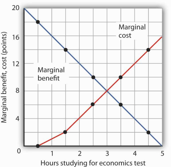
Figure 6.3 shows the marginal cost curve of studying economics. We see that at first, time devoted to studying economics has a low marginal cost. As time spent studying economics increases, however, it requires her to give up study time in accounting that she expects will be more and more productive. The marginal cost curve for studying economics can thus be derived from the marginal benefit curve for studying accounting. Figure 6.3 also shows the marginal benefit curve for studying economics that we derived in Panel (b) of Figure 6.1.

The marginal benefit curve from Panel (c) of Figure 6.1 is shown together with the marginal costs of studying economics. The marginal cost curve is derived from the marginal benefit curve for studying accounting shown in Figure 6.2.
Just as marginal benefit curves generally slope downward, marginal cost curves generally slope upward, as does the one in Figure 6.3. In the case of allocating time, the phenomenon of rising marginal cost results from the simple fact that, the more time a person devotes to one activity, the less time is available for another. And the more one reduces the second activity, the greater the forgone marginal benefits are likely to be. That means the marginal cost curve for that first activity rises.
Because we now have marginal benefit and marginal cost curves for studying economics, we can apply the marginal decision rule. This rule says that, to maximize the net benefit of an activity, a decision maker should increase an activity up to the point at which marginal benefit equals marginal cost. That occurs where the marginal benefit and marginal cost curves intersect, with 3 hours spent studying economics and 2 hours spent studying accounting.
- 瀏覽次數:3786


