


OEE theory includes in performance losses both the cycle time slowdown and minor stoppages. Also time losses of this category propagate, as stated before, throughout the whole production process.
A first type of performance losses propagation is due to the propagation of minor stoppages and reduced speed among machines in series system. From theoretical point of view, between two machines with the same cycle time1 - and without buffer, minor stoppage and reduced speed propagate completely like as major stoppage. Obviously just a little buffer can mitigate the propagation.
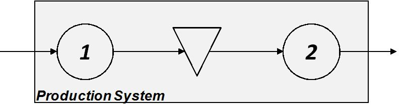
Several models to study the role of buffers in avoiding the propagation of performance losses are available in Buffer Design for Availability literature2. The problem is of scientific relevance, since the lack of opportune buffer between the two stations can indeed affect dramatically the availability of the whole system. To briefly introduce this problem we refer to a production system composed of two consecutive equipments (or stations) with an interposed buffer ( Figure 3.10 ).
Under the likely hypothesis that the ideal cycle times of the two stations are identical3, the variability of speed that affect the stations is not necessarily of the same magnitude, due to its dependence on several factors. Furthermore Performance index is an average of the Tt, therefore a same machine can sometimes perform at a reduced speed and sometimes an highest speed4 - . The presence of this effect in two consecutive equipments can be mutually compensate or add up. Once again, within the propagation analysis for production system design, the role of buffer is dramatically important.
When buffer size is null the system is in series. Hence, as for availability, speed losses of each equipment affect the performance of the whole system:
|
|
Therefore, for the two stations system we can posit:
|
|
But when the buffer is properly designed, it doesn’t allow the minor stoppages and speed losses to propagate from a station to another. We define this Buffer size as Bmax. When, in a production system of n stations, given any couple of consecutive station, the interposed buffer size is Bmax (calculated on the two specific couple of stations), then we have:
|
|
That for the considered 2 stations system is:
|
|
Hence, the extent of the propagation of performance losses depends on the buffer size (j) that is interposed between the two stations. Generally, a bigger buffer increases the performance of the system, since it increases the decoupling degree between two consecutive stations, up to j=Bmax is achieved (j =0,..,Bmax).
We can therefore introduce the parameter
|
|
Considering the model with two station, Figure 3.11 , we have that:
|
|

|
|
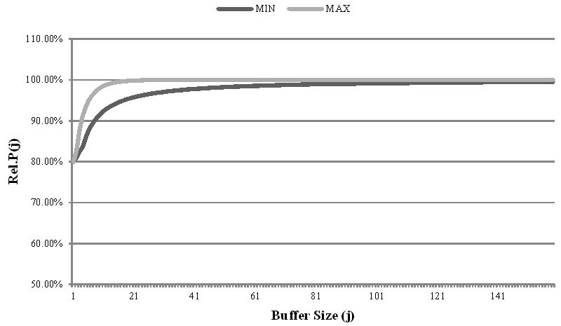
Figure 3.11 shows the trend of Rel.P(j) depending on the buffer size (j), when the performance rate of each station is modeled with an exponential distribution5 in a flow shop environment. The two curves represent the minimum and the maximum simulation results. All the others simulation results are included between these two curves. Maximum curve represents the configuration with the lowest difference in performance index between the two stations, the minimum the configuration with the highest difference.
By analyzing the Figure 3.11 it is clear how an inopportune buffer size affect the performance of the line and how increase in buffer size allows to obtain improve in production line OEE. By the way, once achieved an opportune buffer size no improvement derives from a further increase in buffer. These considerations of Performance index trend are fundamental for an effective design of a production system.
- 5686 reads
