Hazard function

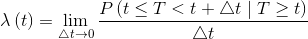
Another very important function is the hazard function, denoted by λ(t), defined as the trend of the instantaneous failure rate at time t of an element that has survived up to that time t. The failure rate is the ratio between the instantaneous probability of failure in a neighborhood of t- conditioned to the fact that the element is healthy in t- and the amplitude of the same neighborhood.

The hazard function λ(t)1 coincides with the intensity function z(t) of a Poisson process. The hazard function is given by:

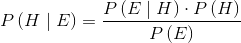
$\lambda \left ( t \right )=\lim_{\triangle t\rightarrow 0}\frac{P\left ( t\leq T< t+\triangle t\mid T\geq t \right )}{\triangle t}$

Thanks to Bayes' theorem, it can be shown that the relationship between the hazard function, density of probability of failure and reliability is the following:

$\lambda \left ( t \right )=\frac{f\left ( t \right )}{R\left ( t \right )}$

Thanks to the previous equation, with some simple mathematical manipulations, we obtain the following relation:

Table 4.6 Equation
$R\left ( t \right )=e^{-\int_{0}^{t}\lambda \left ( u \right )\cdot du}$

In fact, since ln[R(0)]=ln[1]=0, we have:

$R\left ( t \right )=\frac{f\left ( t \right )}{\lambda \left ( t \right )}=\frac{1}{\lambda \left ( t \right )}\cdot \frac{\mathrm{d} F\left ( t \right )}{\mathrm{d} t}=-\frac{1}{\lambda \left ( t \right )}\cdot \frac{\mathrm{d} R\left ( t \right )}{\mathrm{d} t}\rightarrow \frac{1}{R\left ( t \right )}dR\left ( t \right )\\=-\lambda \left ( t \right )dt\rightarrow \ln \left [ R\left ( t \right ) \right ]-\ln \left [ R\left ( 0 \right ) \right ]=-\int_{0}^{t}\lambda \left ( u \right )du$

From Table 4.6 derive the other two fundamental relations:

$F\left ( t \right )=1-e^{-\int_{0}^{t}\lambda \left ( u \right )\cdot du}f\left ( t \right )=\lambda \left ( t \right )\cdot e^{-\int_{0}^{t}\lambda \left ( u \right )\cdot du}$

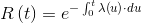
The most popular conceptual model of the hazard function is the bathtub curve. According to this model, the failure rate of the device is relatively high and descending in the first part of the device life, due to the potential manufacturing defects, called early failures. They manifest themselves in the first phase of operation of the system and their causes are often linked to structural deficiencies, design or installation defects. In terms of reliability, a system that manifests infantile failures improves over the course of time.

Later, at the end of the life of the device, the failure rate increases due to wear phenomena. They are caused by alterations of the component for material and structural aging. The beginning of the period of wear is identified by an increase in the frequency of failures which continues as time goes by. Thewear-out failures occur around the average age of operating; the only way to avoid this type of failure is to replace the population in advance.

Between the period of early failures and of wear-out, the failure rate is about constant: failures are due to random events and are called random failures. They occur in non-nominal operating conditions, which put a strain on the components, resulting in the inevitable changes and the consequent loss of operational capabilities. This type of failure occurs during the useful life of the system and corresponds to unpredictable situations. The central period with constant failure rate is called useful life. The juxtaposition of the three periods in a graph which represents the trend of the failure rate of the system, gives rise to a curve whose characteristic shape recalls the section of a bathtub, as shown in Figure 4.12.

Figure 4.12 Bathtub curve

The hazard function shape allows us to identify three areas: the initial period of the early failures, the middle time of the useful life and the final area of wear-out.

The most common mathematical classifications of the hazard curve are the so called Constant Failure Rate - CFR, Increasing Failure Rate - IFR and Decreasing Failure Rate - DFR.

The CFR model is based on the assumption that the failure rate does not change over time. Mathematically, this model is the most simple and is based on the principle that the faults are purely random events. The IFR model is based on the assumption that the failure rate grows up over time. The model assumes that faults become more likely over time because of wear, as is frequently found in mechanical components. The DFR model is based on the assumption that the failure rate decreases over time. This model assumes that failures become less likely as time goes by, as it occurs in some electronic components.

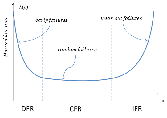
Since the failure rate may change over time, one can define a reliability parameter that behaves as if there was a kind of counter that accumulates hours of operation. The residual reliability function R(t+t₀|t₀), in fact, measures the reliability of a given device which has already survived a determined time t₀. The function is defined as follows:

$R\left ( t+t_{0}\mid t_{0} \right )=P\left ( T> t+t_{0}\mid T> t_{0} \right )$

Applying Bayes' theorem we have:

$P\left ( T> t+t_{0}\mid T> t_{0} \right )=\frac{P\left ( T> t_{0}\mid T> t+t_{0} \right )\cdot P\left ( T> t+t_{0} \right )}{P\left ( Y> t_{0} \right )}$

And, given that P(T>t₀|T>t+t₀)=1, we obtain the final expression, which determines the residual reliability:

$R\left ( t+t_{0}\mid t_{0} \right )=\frac{R\left ( t+t_{0} \right )}{R\left ( t_{0} \right )}$

The residual Mean Time To Failure – residual MTTF measures the expected value of the residual life of a device that has already survived a time t0:

$MTTF\left ( t_{0} \right )=E\left ( T- t_{0}\mid T> t_{0} \right )=\int_{0}^{\infty }R\left ( t+t_{0}\mid t_{0} \right )\cdot dt$

For an IFR device, the residual reliability and the residual MTTF, decrease progressively as the device accumulates hours of operation. This behavior explains the use of preventive actions to avoid failures. For a DFR device, both the residual reliability and the residual MTTF increase while the device accumulates hours of operation. This behavior motivates the use of an intense running (burn-in) to avoid errors in the field.

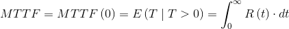
The Mean Time To Failure –MTTF, measures the expected value of the life of a device and coincides with the residual time to failure, where t₀=0. In this case we have the following relationship:

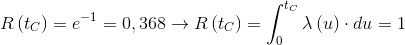
$MTTF=MTTF\left ( 0 \right )=E\left ( T\mid T> 0 \right )=\int_{0}^{\infty }R\left ( t \right )\cdot dt$

The characteristic life of a device is the time t_C corresponding to a reliability R(t_C) equal to 1/e, that is the time for which the area under the hazard function is unitary:

$R\left ( t_{C} \right )=e^{-1}=0,368\rightarrow R\left ( t_{C} \right )=\int_{0}^{t_{C}}\lambda \left ( u \right )\cdot du=1$

Let us consider a CFR device with a constant failure rate λ. The time-to-failure is an exponential random variable. In fact, the probability density function of a failure, is typical of an exponential distribution:

$f\left ( t \right )=\lambda \left ( t \right )\cdot e^{-\int_{0}^{t}\lambda \left ( u \right )\cdot du}=\lambda e^{-\lambda \cdot t}$

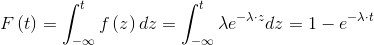
The corresponding cumulative distribution function F(t) is:

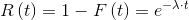
$F\left ( t \right )=\int_{-\infty }^{t}f\left ( z \right )dz=\int_{-\infty }^{t}\lambda e^{-\lambda \cdot z}dz=1-e^{-\lambda \cdot t}$

The reliability function R(t) is the survival function:

$R\left ( t \right )=1-F\left ( t \right )=e^{-\lambda \cdot t}$

For CFR items, the residual reliability and the residual MTTF both remain constant when the device accumulates hours of operation. In fact, from the definition of residual reliability, ∀t₀∈[0,∞], we have:

$R\left ( t+t_{0}\mid t_{0} \right )=\frac{R\left ( t+t_{0} \right )}{R\left ( t_{0} \right )}=\frac{e^{-\lambda \cdot \left ( t+t_{0} \right )}}{e^{-\lambda \cdot t_{0}}}=e^{-\lambda \cdot \left ( t+t_{0} \right )+\lambda \cdot t_{0}}=e^{-\lambda \cdot t}=R\left ( t \right )$

Similarly, for the residual MTTF, is true the invariance in time:

$MTTF\left ( t_{0} \right )=\int_{0}^{\infty }R\left ( t+t_{0}\mid t_{0} \right )\cdot dt=\int_{0}^{\infty }R\left ( t \right )\cdot dt\; \; \; \; \; \; \; \forall t_{0}\; \in \left [ 0,\infty \right ]$

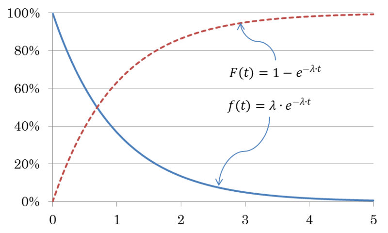
This behavior implies that the actions of prevention and running are useless for CFR devices. Figure 4.13 shows the trend of the function f(t)=λ∙e^−λ∙t and of the cumulative distribution function F(t)=1−e^−λ∙t for a constant failure rate λ=1. In this case, since λ=1, the probability density function and the reliability function, overlap: f(t)=R(t)=e^−t.

Figure 4.13 Probability density function and cumulative distribution of an exponential function

In the figure is seen the trend of f(t)=λ∙e^−λ∙t and of f(t)=λ∙e^−λ∙t with λ=1.

The probability of having a fault, not yet occurred at time t, in the next dt, can be written as follows:

$P\left ( t< T< t+dt\mid T> t \right )$

Recalling the Bayes' theorem, in which we consider the probability of an hypothesis H, being known the evidence E:

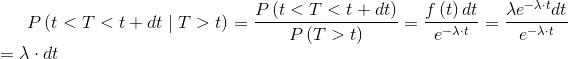
$P\left ( H\mid E \right )=\frac{P\left ( E\mid H \right )\cdot P\left ( H \right )}{P\left ( E \right )}$

we can replace the evidence E with the fact that the fault has not yet taken place, from which we obtain P(E)→P(T>t). We also exchange the hypothesis H with the occurrence of the fault in the neighborhood of t, obtaining P(H)→ P(t<T<t+dt). So we get:

$P\left ( t< T< t+dt\mid T> t \right )=\frac{P\left ( T> t\mid t< T< t+dt \right )\cdot P\left ( t< T< t+dt \right )}{P\left ( T> t \right )}$

Since P(T>t|t<T<t+dt)=1, being a certainty, it follows:

$P\left ( t< T< t+dt\mid T> t \right )=\frac{P\left ( t< T< t+dt \right )}{P\left ( T> t \right )}=\frac{f\left ( t \right )dt}{e^{-\lambda \cdot t}}=\frac{\lambda e^{-\lambda \cdot t}dt}{e^{-\lambda \cdot t}}\\=\lambda \cdot dt$

As can be seen, this probability does not depend on t, i.e. it is not function of the life time already elapsed. It is as if the component does not have a memory of its own history and it is for this reason that the exponential distribution is called memoryless.

The use of the constant failure rate model, facilitates the calculation of the characteristic life of a device. In fact for a CFR item, tCis the reciprocal of the failure rate. In fact:

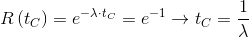
$R\left ( t_{C} \right )= e^{-\lambda \cdot t_{C}}=e^{-1}\rightarrow t_{C}= \frac{1}{\lambda }$

Therefore, the characteristic life, in addition to be calculated as the time value t_C for which the reliability is 0.368, can more easily be evaluated as the reciprocal of the failure rate.

The definition of MTTF, in the CFR model, can be integrated by parts and give:

$MTTF=\int_{0}^{\infty }R\left ( t \right )\cdot dt=\int_{0}^{\infty }e^{-\lambda \cdot t}\cdot dt=-\frac{1}{}\lambda e^{-\lambda \cdot t} \mid \begin{matrix} \infty \\ 0 \end{matrix}=-\frac{0}{\lambda }+\frac{1}{\lambda }=\frac{1}{\lambda }$

In the CFR model, then, the MTTF and the characteristic life coincide and are equal to 1/λ.

Let us consider, for example, a component with constant failure rate equal to λ=0.0002failures per hour. We want to calculate the MTTF of the component and its reliability after 10000 hours of operation. We’ll calculate, then, what is the probability that the component survives other 10000hours. Assuming, finally, that it has worked without failure for the first 6000 hours, we’ll calculate the expected value of the remaining life of the component.

From Table we have:

$MTTF=\frac{1}{\lambda }=\frac{1}{0.0002\left [ \frac{failures}{h} \right ]}=5000\left [ h \right ]$

For the law of the reliability R(t)=e^−λ∙t, you get the reliability at 10000 hours:

$R\left ( 10000 \right )=e^{-0.0002\cdot 10000}=0.135$

The probability that the component survives other 10000 hours, is calculated with the residual reliability. Knowing that this, in the model CFR, is independent from time, we have:

$R\left ( t+ t_{0}\mid t_{0} \right )=R\left ( t \right )\rightarrow R\left ( 20000\mid 10000 \right )=R\left ( 10000 \right )=0.135$

Suppose now that it has worked without failure for 6000 hours. The expected value of the residual life of the component is calculated using the residual MTTF, that is invariant. In fact:

$MTTF\left ( t_{0} \right )=\int_{0}^{\infty }R\left ( t+t_{0} \mid t_{0}\right )\cdot dt\rightarrow MTTF\left ( 6000 \right )\\=\int_{0}^{\infty }R\left ( t+6000\mid 6000 \right )\cdot dt=\int_{0}^{\infty }R\left ( t \right )\cdot dt=MTTF=5000\left [ h \right ]$

4492 reads

You are here

Hazard function