MAINTENANCE AVAILABILITY

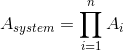
The availability of an equipment1 is defined as $A_{eff}=\frac{T_{u}}{T_{t}}$ . The availability of the whole production system can be defined similarly. Nevertheless it depends upon the equipment configurations. Operations Manager, through the choice of equipment configurations can increase the maintenance availability. This is a design decision, since different equipments must be bought and installed according to desired availability level. The choice of the configuration usually results as a trade-off between equipment costs and system availability. The two main equipment configuration (not-redundant system, redundant system) are debated in the following.

Not redundant system

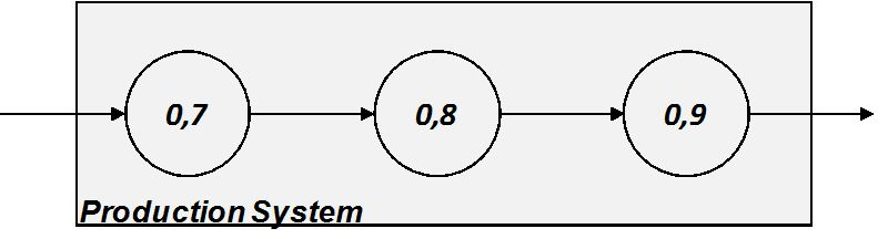
When a system is composed of non redundant equipment, each station produces only if the equipment is working.

Hence if we consider a line of n equipment connected a s a series we have that the downtime of each equipment causes the downtime of the whole system.

$A_{system}= \prod_{i= 1}^{n} A_{i}$

$A_{system}= \prod_{i= 1}^{n} A_{i}= 0,7\ast 0,8\ast 0,9= 0,504$

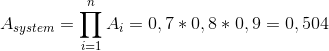
The availability of system composed of a series of equipment is always lower than the availability of each equipment ( Figure 3.6 ).

Figure 3.6 Availability of not redundant System

Total redundant system

Oppositely, to avoid failure propagation amid stations, designer can set the line with a total redundancy of a given equipment. In this case only the contemporaneous downtime of both equipments causes the downtime of the whole system.

$A_{system}= 1-\prod_{i= 1}^{n}\left ( 1-A_{i} \right )$

In the example in Figure 3.7 we have two single equipments connected with a redundant system of two equipment (dotted line system).

Hence, the redundant system availability (dotted line system) rises from 0,8 (of the single equipment) up to:

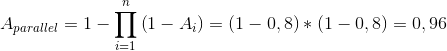
$A_{parallel}= 1-\prod_{i= 1}^{n}\left ( 1-A_{i} \right )= \left ( 1-0,8 \right )\ast \left ( 1-0,8 \right )= 0,96$

Consequently the availability of the whole system will be:

$A_{system}= \prod_{i= 1}^{n}A_{i}= 0,7\ast \left [ 0,96 \right ]\ast 0,9= 0,6048$

Figure 3.7 Availability of totally redundant equipments connected with not redundant equipments

To achieve an higher level of availability it has been necessary to buy two identical equipments (double cost). Hence, the higher value of availability of the system should be worth economically.

Partial redundancy

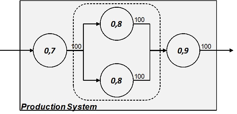
An intermediate solution can be the partial redundancy of an equipment. This is named K/n system, where n is the total number of equipment of the parallel system and k is the minimum number of the nequipment that must work properly to ensure the throughput is produced. The Figure 3.8 shows an example.

The capacity of equipment b’, b’’ and b’’’ is 50 pieces in the referral time unit. If the three systems must ensure a throughput of 100 pieces, it is at least necessary that k=2 of the n=3 equipment produce 50 pieces. The Table 3.7 shows the configuration states which ensure the output is produced and the relative probability that each state manifests.

Figure 3.8 Availability of partially redundant equipments connected with not redundant equipments

Table 3.7 State Analysis Configuration
b’	b’’	b’’’	Probability of occurrance	[*100]
UP	UP	UP	0,80,80,8	0,512
UP	UP	DOWN	0,80,8(1-0,8)	0,128
UP	DOWN	UP	0,8(1-0,8)0,8	0,128
DOWN	UP	UP	(1-0,8)0,80,8	0,128
Total Availability				0,896

In this example all equipments b have the same reliability (0,8), hence the probability the system of three equipment ensure the output should have been calculated, without the state analysis configuration ( Table 3.7 ), through the binomial distribution:

$R_{k/n}= \sum_{j= k}^{n}\binom{n}{j}R^{j}\left [ 1-R \right ]^{n-j}$

$R_{2/3}= \binom{3}{2}0,8^{2}\left [ 1-0,8 \right ]+\binom{3}{3}0,8^{3}= 0,896$

Hence, the availability of the system (a, b’-b’’-b’’’, c) will be:

$A_{system}= \prod_{i= 1}^{n}A_{i}= 0,7\ast \left [ 0,896 \right ]\ast 0,9= 0,56448$

In this case the investment in redundancy is lower than the previous. It is clear how the choice of the level of availability is a trade-off between fix-cost (due to equipment investment) and lack of availability.

In all the cases we considered the buffer as null.

When reliability of the equipments (b in our example) the binomial distribution (16) is not applicable, therefore the state analysis configuration ( Table 3.7 ) is required.

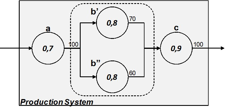
Redundancy with modular capacity

Another configuration is possible.

The production system can be designed as composed of two equipment which singular capacity is lower than the requested but which sum is higher. In this case if it is possible to modulate the production capacity of previous and successive stations the expected throughput will be higher than the output of a singular equipment.

Considering the example in Figure 3.9 when b’ and b’’ are both up the throughput of the subsystem b’-b’’ is 100, since capacity of a and c is 100. Supposing that capacity of a and c is modular, when b’ is down the subsystem can produce 60 pieces in the time unit. Similarly, when b’’ is down the subsystem can produce 70. Hence, the expected amount of pieces produced by b’-b’’ is 84,8 pieces ( Table 3.8 ).

When considering the whole system if either a or c are down the system cannot produce. Hence, the expected throughput in the considered time unit must be reduced of the availability of the two equipments:

Figure 3.9 Availability of partially redundant equipments connected with not redundant equipments at modular capacity

Table 3.8 State Analysis Configuration
b’	b’’	Maximum Throughput	Probability of occurrence	[*100]	Expected Pieces Produced
UP	UP	100	0,8*0,8	0,64	64
UP	DOWN	70	0,8*(1-0,8)	0,16	11,2
DOWN	UP	60	(1-0,8)*0,8	0,16	9,6
	Expected number of Pieces Produced				84,8

1808 reads

You are here

MAINTENANCE AVAILABILITY