


The marginal decision rule, as it applies to a firm’s use of factors, calls for the firm to add more units of a factor up to the point that the factor’s MRP is equal to its MFC. Figure 14.3 illustrates this solution for a firm that is the only buyer of labor in a particular market.
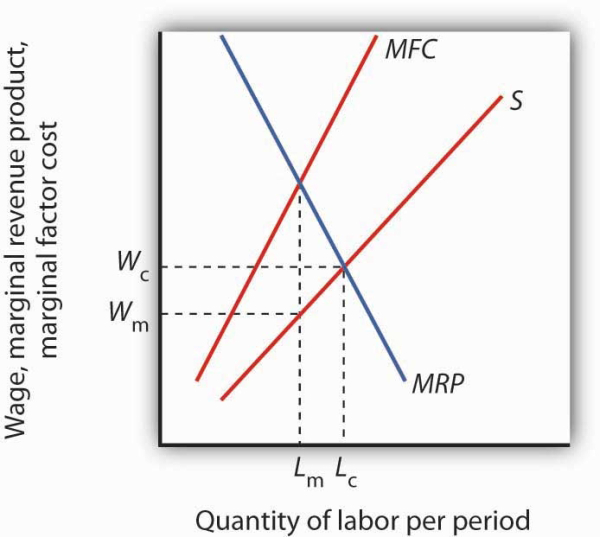
Given the supply curve for labor, S, and the marginal factor cost curve, MFC, the monopsony firm will select the quantity of labor at which the MRPof labor equals its MFC. It thus uses Lm units of labor (determined by at the intersection of MRPand MFC) and pays a wage of Wmper unit (the wage is taken from the supply curve at which Lm units of labor are available). The quantity of labor used by the monopsony firm is less than would be used in a competitive market (Lc); the wage paid, Wm, is lower than would be paid in a competitive labor market.
The firm faces the supply curve for labor, S, and the marginal factor cost curve for labor, MFC. The profit-maximizing quantity is determined by the intersection of the MRP and MFC curves—the firm will hire Lm units of labor. The wage at which the firm can obtain Lm units of labor is given by the supply curve for labor; it is Wm. Labor receives a wage that is less than its MRP.
If the monopsony firm was broken up into a large number of small firms and all other conditions in the market remained unchanged, then the sum of the MRP curves for individual firms would be the market demand for labor. The equilibrium wage would be Wc, and the quantity of labor demanded would be Lc. Thus, compared to a competitive market, a monopsony solution generates a lower factor price and a smaller quantity of the factor demanded.
- 5831 reads
