


When we draw a graph showing the relationship between two variables, we make an important assumption. We assume that all other variables that might affect the relationship between the variables in our graph are unchanged. When one of those other variables changes, the relationship changes, and the curve showing that relationship shifts.
Consider, for example, the ski club that sponsors bus trips to the ski area. The graph we drew in Figure 20.4 shows the relationship between club revenues from a particular trip and the number of passengers on that trip, assuming that all other variables that might affect club revenues are unchanged. Let us change one. Suppose the school’s student government increases the payment it makes to the club to $400 for each day the trip is available. The payment was $200 when we drew the original graph. Panel (a) of Figure 20.8 shows how the increase in the payment affects the table we had in Figure 20.3; Panel (b) shows how the curve shifts. Each of the new observations in the table has been labeled with a prime: A′, B′, etc. The curve R1 shifts upward by $200 as a result of the increased payment. A shift in a curveimplies new values of one variable at each value of the other variable. The new curve is labeled R2. With 10 passengers, for example, the club’s revenue was $300 at point B on R1. With the increased payment from the student government, its revenue with 10 passengers rises to $500 at point B′ on R2. We have a shift in the curve.
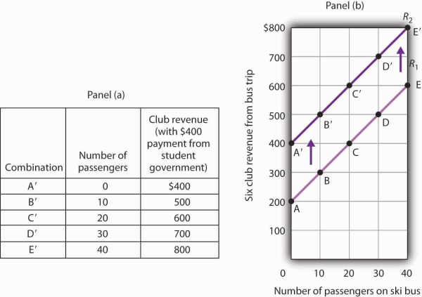
The table in Panel (a) shows the new level of revenues the ski club receives with varying numbers of passengers as a result of the increased payment from student government. The new curve is shown in dark purple in Panel (b). The old curve is shown in light purple.
It is important to distinguish between shifts in curves and movements along curves. A movement along a curve is a change from one point on the curve to another that occurs when the dependent variable changes in response to a change in the independent variable. If, for example, the student government is paying the club $400 each day it makes the ski bus available and 20 passengers ride the bus, the club is operating at point C′ on R2. If the number of passengers increases to 30, the club will be at point D′ on the curve. This is a movement along a curve; the curve itself does not shift.
Now suppose that, instead of increasing its payment, the student government eliminates its payments to the ski club for bus trips. The club’s only revenue from a trip now comes from its $10/passenger charge. We have again changed one of the variables we were holding unchanged, so we get another shift in our revenue curve. The table in Panel (a) of Figure 20.8 shows how the reduction in the student government’s payment affects club revenues. The new values are shown as combinations A″ through E″ on the new curve, R3, in Panel (b). Once again we have a shift in a curve, this time from R1 to R3.
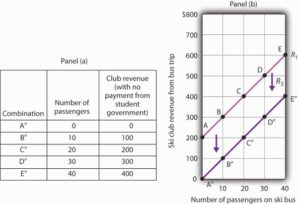
The table in Panel (a) shows the impact on ski club revenues of an elimination of support from the student government for ski bus trips. The club’s only revenue now comes from the $10 it charges to each passenger. The new combinations are shown as A″ – E″. In Panel (b) we see that the original curve relating club revenue to the number of passengers has shifted down.
The shifts in Figure 20.8 and Figure 20.9 left the slopes of the revenue curves unchanged. That is because the slope in all these cases equals the price per ticket, and the ticket price remains unchanged. Next, we shall see how the slope of a curve changes when we rotate it about a single point.
- 1157 reads
