


Changes in demand can occur for a variety of reasons. There may be a change in preferences, incomes,the price of a related good, population, or consumer expectations. A change in demand causes a change in the market price, thus shifting the marginal revenue curves of firms in the industry.
Let us consider the impact of a change in demand for oats. Suppose new evidence suggests that eating oats not only helps to prevent heart disease, but also prevents baldness in males. This will, of course, increase the demand for oats. To assess the impact of this change, we assume that the industry is perfectly competitive and that it is initially in long-run equilibrium at a price of $1.70 per bushel.
Economic profits equal zero.
The initial situation is depicted in Figure 9.15. Panel (a) shows that at a price of $1.70, industry output is Q1 (point A), while Panel (b) shows that the market price constitutes the marginal revenue,MR1, facing a single firm in the industry. The firm responds to that price by finding the output level atwhich the MC and MR1 curves intersect. That implies a level of output q1 at point A′.
The new medical evidence causes demand to increase to D2 in Panel (a). That increases the market price to $2.30 (point B), so the marginal revenue curve for a single firm rises to MR2 in Panel (b). The firm responds by increasing its output to q2 in the short run (point B′). Notice that the firm’s averagetotal cost is slightly higher than its original level of $1.70; that is because of the U shape of the curve.The firm is making an economic profit shown by the shaded rectangle in Panel (b). Other firms in the industry will earn an economic profit as well, which, in the long run, will attract entry by new firms.
New entry will shift the supply curve to the right; entry will continue as long as firms are making an economic profit. The supply curve in Panel (a) shifts to S2, driving the price down in the long run to the original level of $1.70 per bushel and returning economic profits to zero in long-run equilibrium. A single firm will return to its original level of output, q1 (point A′) in Panel (b), but because there are more firms in the industry, industry output rises to Q3 (point C) in Panel (a).
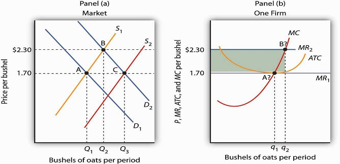
The initial equilibrium price and output are determined in the market for oats by the intersection of demand and supply at point A in Panel (a). An increase in the market demand for oats, from D1 to D2 in Panel (a), shifts the equilibrium solution to point B. The price increases in the short run from $1.70 per bushel to $2.30. Industry output rises to Q2. For a single firm, the increase in price raises marginal revenue from MR1 to MR2; the firm responds in the short run by increasing its output to q2. It earns an economic profit given by the shaded rectangle. In the long run,the opportunity for profit attracts new firms. In a constant-cost industry, the short-run supply curve shifts to S2;market equilibrium now moves to point C in Panel (a). The market price falls back to $1.70. The firm’s demand curve returns to MR1, and its output falls back to the original level, q1. Industry output has risen to Q3 because there are more firms.
A reduction in demand would lead to a reduction in price, shifting each firm’s marginal revenue curvedownward. Firms would experience economic losses, thus causing exit in the long run and shifting the supply curve to the left. Eventually, the price would rise back to its original level, assuming changes inindustry output did not lead to changes in input prices. There would be fewer firms in the industry, but each firm would end up producing the same output as before.
- 2387 reads
