


Next time you purchase an item at a store, notice the sales tax imposed by your state, county, and city.The clerk rings up the total, then adds up the tax. The store is the entity that “pays” the sales tax, in the sense that it sends the money to the government agencies that imposed it, but you are the one who actually foots the bill—or are you? Is it possible that the sales tax affects the price of the item itself?
These questions relate to tax incidence analysis, a type of economic analysis that seeks to determine where the actual burden of a tax rests. Does the burden fall on consumers, workers, owners of capital, owners of natural resources, or owners of other assets in the economy? When a tax imposed on a good or service increases the price by the amount of the tax, the burden of the tax falls on consumers. If instead it lowers wages or lowers prices for some of the other factors of production used in the production of the good or service taxed, the burden of the tax falls on owners of these factors. If the tax does not change the product’s price or factor prices, the burden falls on the owner of the firm—the owner of capital. If prices adjust by a fraction of the tax, the burden is shared.
Figure 15.6 gives an example of tax incidence analysis. Suppose D1 and S1 are the demand and supply curves for beef. The equilibrium price is $3 per pound; the equilibrium quantity is 3 million pounds of beef per day. Now suppose an excise tax of $2 per pound of beef is imposed. It does not matter whether the tax is levied on buyers or on sellers of beef; the important thing to see is that the tax drives a $2 per pound “wedge” between the price buyers pay and the price sellers receive. This tax is shown as the vertical green line in the exhibit; its height is $2.
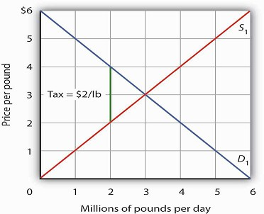
Suppose the market price of beef is $3 per pound; the equilibrium quantity is 3 million pounds per day. Now suppose an excise tax of $2 per pound is imposed, shown by the vertical green line. We insert this tax wedge between the demand and supply curves. It raises the market price to $4 per pound, suggesting that buyers pay half the tax in the form of a higher price. Sellers receive a price of $2 per pound; they pay half the tax by receiving a lower price. The equilibrium quantity falls to 2 million pounds per day.
We insert our tax “wedge” between the demand and supply curves. In our example, the price paid by buyers rises to $4 per pound. The price received by sellers falls to $2 per pound; the other $2 goes to the government. The quantity of beef demanded and supplied falls to 2 million pounds per day. In this case, we conclude that buyers bear half the burden of the tax (the price they pay rises by $1 per pound), and sellers bear the other half (the price they receive falls by $1 per pound). In addition to the change in price, a further burden of the tax results from the reduction in consumer and in producer surplus. We have not shown this reduction in the graph.
Figure 15.7 shows how tax incidence varies with the relative elasticities of demand and supply. All four panels show markets with the same initial price, P1, determined by the intersection of demand D1 and supply S1. We impose an excise tax, given by the vertical green line. As before, we insert this tax wedge between the demand and supply curves. We assume the amount of the tax per unit is the same in each of the four markets.
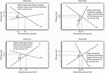
We show the effect of an excise tax, given by the vertical green line, in the same way that we did in Figure 15.6. We see that buyers bear most of the burden of such a tax in cases of relatively elastic supply (Panel (a)) and of relatively inelastic demand (Panel (d)). Sellers bear most of the burden in cases of relatively inelastic supply (Panel (b)) and of relatively elastic demand (Panel (c)).
In Panel (a), we have a market with a relatively elastic supply curve S1. When we insert our tax wedge,the price rises to P2; the price increase is nearly as great as the amount of the tax. In Panel (b), we have the same demand curve as in Panel (a), but with a relatively inelastic supply curve S2. This time the price paid by buyers barely rises; sellers bear most of the burden of the tax. When the supply curve is relatively elastic, the bulk of the tax burden is borne by buyers. When supply is relatively inelastic, the bulk of the burden is borne by sellers.
Panels (c) and (d) of the exhibit show the same tax imposed in markets with identical supply curves S1. With a relatively elastic demand curve D1 in Panel (c) (notice that we are in the upper half, that is, the elastic portion of the curve), most of the tax burden is borne by sellers. With a relatively inelastic demand curve D1 in Panel (d) (notice that we are in the lower half, that is, the inelastic portion of the curve), most of the burden is borne by buyers. If demand is relatively elastic, then sellers bear more of the burden of the tax. If demand is relatively inelastic, then buyers bear more of the burden.
The Congressional Budget Office (CBO) has prepared detailed studies of the federal tax system. Using the tax laws in effect in August 2004, it ranked the U.S. population according to ncome and then divided the population into quintiles (groups containing 20% of the population). Then, given the federal tax burden imposed by individual income taxes, payroll taxes for social insurance, corporate income taxes, and excise taxes on each quintile and the income earned by people in that quintile, it projected the average tax rate facing that group in 2006. The study assigned taxes on the basis of who bears the burden, not on who pays the tax. For example, many studies argue that, even though businesses pay half of the payroll taxes, the burden of payroll taxes actually falls on households. The reason is that the supply curve of labor is relatively inelastic, as shown in Panel (b) of Figure 15.7. Taking these adjustments into account, the CBO’s results, showing progressivity in federal taxes, are reported in the following Table 15.2.
In a regressive tax system, people in the lowest quintiles face the highest tax rates. A proportional system imposes the same rates on everyone; a progressive system imposes higher rates on people in higher deciles. The table gives estimates by the CBO of the burden on each quintile of federal taxes in 2006. As you can see, the tax structure in the United States is progressive.
|
Income category |
Households (number, millions) |
Average Pretax comprehensive household income |
Effective federal tax rate, 2006 (percent) |
|---|---|---|---|
|
Lowest quintile |
24.0 |
$18,568 |
5.6 |
|
Second quintile |
22.8 |
$42,619 |
12.1 |
|
Middle quintile |
23.3 |
$64,178 |
15.7 |
|
Fourth quintile |
23.2 |
$94,211 |
19.8 |
|
Highest |
24.3 |
$227,677 |
26.5 |
Source: CBO, Effective Federal Tax Rates under Current Law, 2001 to 2014, August, 2004, Table 2 and Table A-1 (adjusted by authors using CBO assumptions concerning rates of growth of income and households). Numbers of households do not add up to total because of excluded categories. Quintiles contains equal numbers of people.
KEY TAKEAWAYS
- The primary principles of taxation are the ability-to-pay and benefits-received principles.
- The percentage of income taken by a regressive tax rises as income falls. A proportional tax takes a constant percentage of income regardless of income level. A progressive tax takes a higher percentage of income as taxes as incomes rise.
- The marginal tax rate is the tax rate that applies to an additional dollar of income earned.
- Tax incidence analysis seeks to determine who ultimately bears the burden of a tax.
- The major types of taxes are income taxes, sales taxes, property taxes, and excise taxes.Buyers bear most of the burden of an excise tax when supply is relatively elastic and when demand is relatively inelastic; sellers bear most of the burden when supply is relatively inelastic and when demand is relatively elastic.
- The federal tax system in the United States is progressive.
TRY IT!
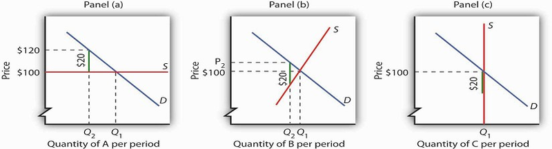
Consider three goods, A, B, and C. The prices of all three goods are determined by demand and supply (that is, the three industries are perfectly competitive) and equal $100. The supply curve for good A is perfectly elastic; the supply curve for good B is a typical, upward-sloping curve; and the supply curve for good C is perfectly inelastic. Suppose the federal government imposes a tax of $20 per unit on suppliers of each good. Explain and illustrate graphically how the tax will affect the price of each good in the short run. Show whether the equilibrium quantity will rise, fall, or remain unchanged. Who bears the burden of the tax on each good in the short run? (Hint: Review the chapter on the elasticity for a discussion of perfectly elastic and perfectly inelastic supply curves; remember that the tax increases variable cost by $20 per unit.)
Case in Point
We speak often of the importance of tax rates at the margin—of how much of an extra dollar earned through labor or interest on saving will be kept by the decision-maker. It turns out,
however, that figuring out just what that marginal tax rate is is not an easy task.
Consider the difficulty of untangling just what those marginal tax rates are. First, Americans face a bewildering complex of taxes. They all face the federal income tax. Each state—and many
cities—levy additional taxes on income. Then there is the FICA payroll tax, federal and state corporate income taxes, and excise taxes, as well as federal, state, and local sales taxes. A
person trying to figure out his or her marginal tax rate cannot stop there. Gaining an additional dollar of income will affect not only taxes but eligibility for various transfer payment
programs in the level of payments the individual or household can expect to receive. Given the enormous complexity involved, it is safe to say that no one really knows what his or her
marginal rate is.
Economists Laurence J. Kotlikoff and David Rapson of Boston University have taken on the task of sorting outmarginal tax rates for the United States. They used a commercial tax analysis
program, Economic Security Planner ™, and added their own computer programs to incorporate the effect of additional income on various transfer payment programs. Their analysis assumed the
taxpayer lived in Massachusetts, but the general tenor of their results applies to people throughout the United States.
Consider a 60-year-old couple earning $10,000 per year. That couple is eligible for a variety of welfare programs. With food stamps, there is a dollar-for-dollar reduction in aid for each
additional dollar of income earned. In effect, the couple faces an effective marginal tax rate of 100%. Considering all other taxes and welfare programs, the economists concluded that the
couple faced a marginal tax rate of about 50% on labor income. Overall, they found that a pattern of marginal rates for various ages and income levels could be described in a single word:
“bizarre.”
The tables below give the economists’ estimates of marginal rates for current year labor supply for a single individual and for couples with children at various incomes and ages. While the
overall structure of taxes in the United States is progressive, the special treatment of welfare programs can add a strong element of regressivity.
|
Marginal Net Tax Rates on Current-Year Labor Supply (Couples, percentages) |
|||||
|---|---|---|---|---|---|
|
Total Annual Household Earnings (000s) |
|||||
|
Age |
10 |
20 |
30 |
50 |
75 |
|
30 |
-14.2 |
42.5 |
42.3 |
24.4 |
36.9 |
|
45 |
-11.4 |
41.7 |
41.8 |
35.8 |
36.1 |
|
60 |
50.9 |
32.0 |
36.3 |
36.3 |
45.5 |
|
Age |
100 |
150 |
200 |
300 |
500 |
|
30 |
37.0 |
45.9 |
36.8 |
43.9 |
44.0 |
|
45 |
36.1 |
45.1 |
35.9 |
40.0 |
43.2 |
|
60 |
45.5 |
47.7 |
43.2 |
45.8 |
45.0 |
Source: Laurence J. Kotlikoff and David Rapson, “Does It Pay, At the Margin, to Work and Save?” NBER Tax Policy & the Economy, 2007, 21(1): 83–143. The tables shown here are Tables 4.2 and 4.3 in the article.
|
Marginal Net Tax Rates on Current-Year Labor Supply (Individuals, percentages) |
|||||
|---|---|---|---|---|---|
|
Total Annual Household Earnings (000s) |
|||||
|
Age |
10 |
20 |
30 |
50 |
75 |
|
30 |
72.3 |
42.9 |
42.9 |
37.0 |
37.0 |
|
45 |
-0.8 |
42.9 |
42.6 |
37.0 |
36.1 |
|
60 |
39.5 |
37.3 |
37.7 |
46.4 |
45.5 |
|
Age |
125 |
150 |
200 |
250 |
|
|
30 |
36.2 |
36.9 |
42.0 |
41.5 |
|
|
45 |
36.1 |
36.5 |
42.0 |
41.5 |
|
|
60 |
38.8 |
44.0 |
45.0 |
44.0 |
|
Look again at our 60-year-old couple. It faces a very high marginal tax rate. A younger couple with the same income actually faces a negative marginal tax rate—increasing its labor income by
a dollar actually increases its after-tax income by more than a dollar. Why the difference? The economists assumed that the younger couple would have children and thus qualify for a variety
of programs, including the Earned Income Tax Credit. The couple at age 60 still faces the dollar-for-dollar reduction in payments in the Food Stamp program. No one designed these marginal
incentives. They simply emerge from the bewildering mix of welfare and tax programs households face.
ANSWER TO TRY IT! PROBLEM
The tax adds a $20 wedge between the price paid by buyers and received by sellers. In Panel (a), the price rises to $120; the entire burden is borne by buyers. In Panel (c), the price remains $100; sellers receive just $80.Therefore, sellers bear the burden of the tax. In Panel (b), the price rises by less than $20, and the burden is shared by buyers and sellers. The relative elasticities of demand and supply determine whether the tax is borne primarily by buyers or sellers, or shared equally by both groups.
- 8030 reads
