


A firm’s costs change if the costs of its inputs change. They also change if the firm is able to take advantage of a change in technology. Changes in production cost shift the ATC curve. If a firm’s variable costs are affected, its marginal cost curves will shift as well. Any change in marginal cost produces a similar change in industry supply, since it is found by adding up marginal cost curves for individual firms.
Suppose a reduction in the price of oil reduces the cost of producing oil changes for automobiles.We shall assume that the oil-change industry is perfectly competitive and that it is initially in long-run equilibrium at a price of $27 per oil change, as shown in Panel (a) of Figure 9.16. Suppose that the reduction in oil prices reduces the cost of an oil change by $3.
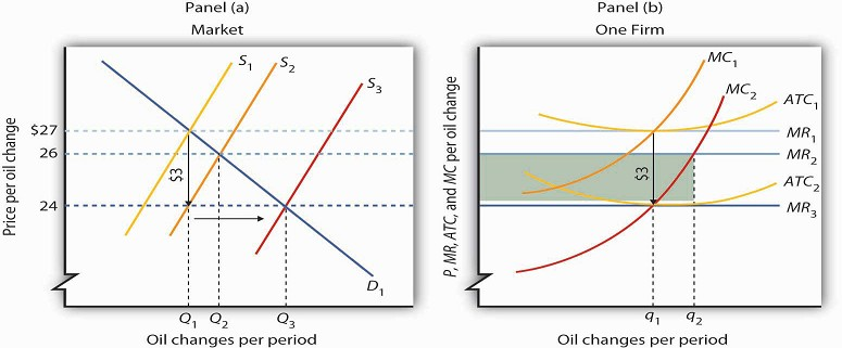
The initial equilibrium price, $27, and quantity, Q1, of automobile oil changes are determined by the intersection of market demand, D1, and market supply, S1 in Panel (a). The industry is in long-run equilibrium; a typical firm, shown in Panel (b), earns zero economic profit. A reduction in oil prices reduces the marginal and average total costs of producing an oil change by $3. The firm’s marginal cost curve shifts to MC2, and its average total cost curve shifts to ATC2. The short-run industry supply curve shifts down by $3 to S2. The market price falls to $26; the firm increases its output to q2 and earns an economic profit given by the shaded rectangle. In the long run, the opportunity for profit shifts the industry supply curve to S3. The price falls to $24, and the firm reduces its output to the original level, q1. It now earns zero economic profit once again. Industry output in Panel (a) rises to Q3 because there are more firms;price has fallen by the full amount of the reduction in production costs.
A reduction in production cost shifts the firm’s cost curves down. The firm’s average total cost and marginal cost curves shift down, as shown in Panel (b). In Panel (a) the supply curve shifts from S1 to S2. The industry supply curve is made up of the marginal cost curves of individual firms; because each of them has shifted downward by $3, the industry supply curve shifts downward by $3.
Notice that price in the short run falls to $26; it does not fall by the $3 reduction in cost. That is because the supply and demand curves are sloped. While the supply curve shifts downward by $3, its intersection with the demand curve falls by less than $3. The firm in Panel (b) responds to the lower price and lower cost by increasing output to q2, where MC2 and MR2 intersect. That leaves firms in the industry with an economic profit; the economic profit for the firm is shown by the shaded rectangle in Panel (b). Profits attract entry in the long run, shifting the supply curve to the right to S3 in Panel (a)Entry will continue as long as firms are making an economic profit—it will thus continue until the price falls by the full amount of the $3 reduction in cost. The price falls to $24, industry output rises to Q3, and the firm’s output returns to its original level, q1.
An increase in variable costs would shift the average total, average variable, and marginal cost curves upward. It would shift the industry supply curve upward by the same amount. The result in the short run would be an increase in price, but by less than the increase in cost per unit. Firms would experience economic losses, causing exit in the long run. Eventually, price would increase by the full amount of the increase in production cost.
Some cost increases will not affect marginal cost. Suppose, for example, that an annual license feeof $5,000 is imposed on firms in a particular industry. The fee is a fixed cost; it does not affect marginal cost. Imposing such a fee shifts the average total cost curve upward but causes no change in marginalcost. There is no change in price or output in the short run. Because firms are suffering economic losses, there will be exit in the long run. Prices ultimately rise by enough to cover the cost of the fee,leaving the remaining firms in the industry with zero economic profit.
Price will change to reflect whatever change we observe in production cost. A change in variable cost causes price to change in the short run. In the long run, any change in average total cost changes price by an equal amount.
The message of long-run equilibrium in a competitive market is a profound one. The ultimate beneficiariesof the innovative efforts of firms are consumers. Firms in a perfectly competitive world earn zero profit in the long-run. While firms can earn accounting profits in the long-run, they cannot earn economic profits.
KEY TAKEAWAYS
The economic concept of profit differs from accounting profit. The accounting concept deals only withexplicit costs, while the economic concept of profit incorporates explicit and implicit
costs. The existence of economic profits attracts entry, economic losses lead to exit, and in long-run equilibrium, firms in a perfectly competitive industry will earn zero economic
profit.
The long-run supply curve in an industry in which expansion does not change input prices (a constantcostindustry) is a horizontal line. The long-run supply curve for an industry in which
production costs increase as output rises (an increasing-cost industry) is upward sloping. The long-run supply curve for an industry in which production costs decrease as output rises (a
decreasing-cost industry) is downward sloping.
In a perfectly competitive market in long-run equilibrium, an increase in demand creates economic profitin the short run and induces entry in the long run; a reduction in demand creates
economic losses (negative economic profits) in the short run and forces some firms to exit the industry in the long run.
hen production costs change, price will change by less than the change in production cost in the shortrun. Price will adjust to reflect fully the change in production cost in the long
run.
A change in fixed cost will have no effect on price or output in the short run. It will induce entry or exit in the long run so that price will change by enough to leave firms earning zero
economic profit.
TRY IT!
Consider Acme Clothing’s situation in the second Try It! in this chapter. Suppose this situation is typical of firms in the jacket market. Explain what will happen in the market for jackets in the long run, assuming nothing happens to the prices of factors of production used by firms in the industry. What will happen to the equilibrium price? What is the equilibrium level of economic profits?
Case in Point: Competition in the Market for Generic Prescription Drugs
© 2010 Jupiterimages Corporation
Generic prescription drugs are essentially identical substitutes for more expensive brand-name prescription drugs. Since the passage of the Drug Competition and Patent Term Restoration Act of
1984 (commonly referred to as the Hatch-Waxman Act) made it easier for manufacturers to enter the market for generic drugs, the generic drug industry has taken off. Generic drugs represented
19% of the prescription drug industry in1984 and today represent more than half of the industry. U.S. generic sales were $15 billion in 2002 and soared to $192 billion in 2006. In 2006, the
average price of a branded prescription was $111.02 compared to $32.23 for a generic prescription.
A Congressional Budget Office study in the late 1990s showed that entry into the generic drug industry has been the key to this price differential. As shown in the table, when there are one
to five manufacturers selling generic copies of a given branded drug, the ratio of the generic price to the branded price is about 60%. With more than 20 competitors, the ratio falls to about
40%.
The generic drug industry is largely characterized by the attributes of a perfectly competitive market. Competitors have good information about the product and sell identical products. The
largest generic drug manufacturer in the CBO study had a 16% share of the generic drug manufacturing industry, but most generic manufacturers ‘sales constituted only 1% to 5% of the market.
The 1984 legislation eased entry into this market. And, as the model of perfect competition predicts, entry has driven prices down, benefiting consumers to the tune of tens of billions of
dollars each year.
|
Number of Generic Manufacturers of a Given Innovator Drug |
Number of Innovator Drugs in Category |
Avg. Rx Price, All Generic Drugs in Category |
Avg. Rx Price, All Innovator Drugs in Category |
Avg. Ratio of the Generic Price to the Innovator Price for Same Drug |
|---|---|---|---|---|
|
1 to 5 |
34 |
$23.40 |
$37.20 |
0.61 |
|
6 to 10 |
26 |
$26.40 |
$42.60 |
0.61 |
|
11 to 15 |
29 |
$20.90 |
$50.20 |
0.42 |
|
16 to 20 |
19 |
$19.90 |
$45.00 |
0.46 |
|
21 to 24 |
4 |
$11.50 |
$33.90 |
0.39 |
|
Average |
$22.40 |
$43.00 |
0.53 |
Sources: Congressional Budget Office, “How Increased Competition from Generic Drugs Has Affected Prices and Returns in the Pharmaceutical Industry,” July 1998. Available at www.cbo.gov; “Generic Pharmaceutical Industry Anticipates Double-Digit Growth,” PR Newswire, March 17, 2004. Available at www.Prnewswire.com; 2008 Statistical Abstract of the United States, Table 130.
ANSWER TO TRY IT! PROBLEM
The availability of economic profits will attract new firms to the jacket industry in the long run, shifting the market supply curve to the right. Entry will continue until economic profits are eliminated. The price will fall;Acme’s marginal revenue curve shifts down. The equilibrium level of economic profits in the long run is zero.
- 7830 reads
