


How large are inflationary and recessionary gaps? Panel (a) of Figure 22.15 shows potential output versus the actual level of real GDP in the United States since 1960. Real GDP appears to follow potential output quite closely, although you see some periods where there have been inflationary or recessionary gaps. Panel (b) shows the sizes of these gaps expressed as percentages of potential output. The percentage gap is positive during periods of inflationary gaps and negative during periods of recessionary gaps. The economy seldom departs by more than 5% from its potential output.
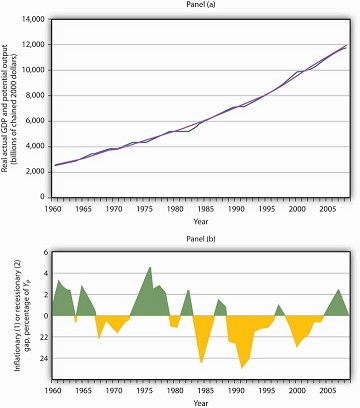
Panel (a) shows potential output (the blue line) and actual real GDP (the purple line) since 1960. Panel (b) shows the gap between potential and actual real GDP expressed as a percentage of potential output. Inflationary gaps are shown in green and recessionary gaps are shown in yellow. Source: Bureau of Economic Analysis, NIPA Table 1.1.6. Real Gross Domestic Product, Chained Dollars [Billions of chained (2000) dollars]. Seasonally adjusted at annual rates 2008 is through 3rd quarter; Congressional Budget Office, The Budget and Economic Outlook, September 9, 2008.
Panel (a) gives a long-run perspective on the economy. It suggests that the economy generally operates at about potential output. In Panel (a), the gaps seem minor. Panel (b) gives a short-run perspective; the view it gives emphasizes the gaps. Both of these perspectives are important. While it is reassuring to see that the economy is often close to potential, the years in which there are substantial gaps have real effects: Inflation or unemployment can harm people.
Some economists argue that stabilization policy can and should be used when recessionary or inflationary gaps exist. Others urge reliance on the economy’s own ability to correct itself. They sometimes argue that the tools available to the public sector to influence aggregate demand are not likely to shift the curve, or they argue that the tools would shift the curve in a way that could do more harm than good.
Economists who advocate stabilization policies argue that prices are sufficiently sticky that the economy’s own adjustment to its potential will be a slow process—and a painful one. For an economy with a recessionary gap, unacceptably high levels of unemployment will persist for too long a time. For an economy with an inflationary gap, the increased prices that occur as the short-run aggregate supply curve shifts upward impose too high an inflation rate in the short run. These economists believe it is far preferable to use stabilization policy to shift the aggregate demand curve in an effort to shorten the time the economy is subject to a gap.
Economists who favor a nonintervention approach accept the notion that stabilization policy can shift the aggregate demand curve. They argue, however, that such efforts are not nearly as simple in the real world as they may appear on paper. For example, policies to change real GDP may not affect the economy for months or even years. By the time the impact of the stabilization policy occurs, the state of the economy might have changed. Policy makers might choose an expansionary policy when a contractionary one is needed or vice versa. Other economists who favor nonintervention also question how sticky prices really are and if gaps even exist.
The debate over how policy makers should respond to recessionary and inflationary gaps is an ongoing one. These issues of nonintervention versus stabilization policies lie at the heart of the macroeconomic policy debate. We will return to them as we continue our analysis of the determination of output and the price level.
KEY TAKEAWAYS
- When the aggregate demand and short-run aggregate supply curves intersect below potential output, the economy has a recessionary gap. When they intersect above potential output, the economy has an inflationary gap.
- Inflationary and recessionary gaps are closed as the real wage returns to equilibrium, where the quantity of labor demanded equals the quantity supplied. Because of nominal wage and price stickiness, however, such an adjustment takes time.
- When the economy has a gap, policy makers can choose to do nothing and let the economy return to potential output and the natural level of employment on its own. A policy to take no action to try to close a gap is a nonintervention policy.
- Alternatively, policy makers can choose to try to close a gap by using stabilization policy. Stabilization policy designed to increase real GDP is called expansionary policy. Stabilization policy designed to decrease real GDP is called contractionary policy.
TRY IT!
Using the scenario of the Great Depression of the 1930s, as analyzed in the previous Try It!, tell what kind of gap the U.S. economy faced in 1933, assuming the economy had been at potential output in 1929. Do you think the unemployment rate was above or below the natural rate of unemployment? How could the economy have been brought back to its potential output?
Case in Point: Survey of Economists Reveals Little Consensus on Macroeconomic Policy Issues
“An economy in short-run equilibrium at a real GDP below potential GDP has a self-correcting mechanism that will eventually return it to potential real GDP.”
Of economists surveyed, 36% disagreed, 33% agreed with provisos, 25% agreed, and 5% did not respond. So, only about 60% of economists responding to the survey agreed that the economy would
adjust on its own.
“Changes in aggregate demand affect real GDP in the short run but not in the long run.” CHAPTER 22 AGGREGATE DEMAND AND AGGREGATE SUPPLY 567
On this statement, 36% disagreed, 31% agreed with provisos, 29% agreed, and 4% did not respond. Once again, about 60% of economists accepted the conclusion of the aggregate demand–aggregate
supply model. This level of disagreement on macroeconomic policy issues among economists, based on a fall 2000 survey of members of the American Economic Association, stands in sharp contrast
to their more harmonious responses to questions on international economics and microeconomics. For example, “Tariffs and import quotas usually reduce the general welfare of society.”
Seventy-two percent of those surveyed agreed with this statement outright and another 21% agreed with provisos. So, 93% of economists generally agreed with the statement.
“Minimum wages increase unemployment among young and unskilled workers.”
On this, 45% agreed and 29% agreed with provisos.
“Pollution taxes or marketable pollution permits are a more economically efficient approach to pollution control than emission standards.”
On this environmental question, only 6% disagreed and 63% wholeheartedly agreed.
The relatively low degree of consensus on macroeconomic policy issues and the higher degrees of consensus on other economic issues found in this survey concur with results of other periodic
surveys since 1976.
So, as textbook authors, we will not hide the dirty laundry from you. Fortunately, though, the model of aggregate demand–aggregate supply we present throughout the macroeconomic chapters can
handle most of these disagreements. For example, economists who agree with the first proposition quoted above, that an economy operating below potential has self-correcting mechanisms to
bring it back to potential, are probably assuming that wages and prices are not very sticky and hence that the short-run aggregate supply curve will shift rather easily to the right, as shown
in Panel (a) of . In contrast, economists who disagree with the statement are saying that the movement of the short-run aggregate supply curve is likely to be slow. This latter group of
economists probably advocates expansionary policy as shown in Panel (b) of Figure 22.13. Both groups of economists can use the same model and its constructs to analyze the macroeconomy, but they may
disagree on such things as the slopes of the various curves, on how fast these various curves shift, and on the size of the underlying multiplier. The model allows economists to speak the
same language of analysis even though they disagree on some specifics.
Source: Dan Fuller and Doris Geide-Stevenson, “Consensus on Economic Issues: A Survey of Republicans, Democrats and Economists,” Eastern Economic Journal 33, no. 1 (Winter 2007):
81–94.
ANSWER TO TRY IT! PROBLEM
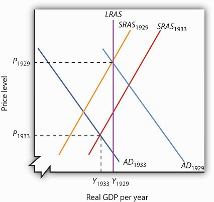
To the graph in the previous Try It! problem we add the long-run aggregate supply curve to show that, with output below potential, the U.S. economy in 1933 was in a recessionary gap. The
unemployment rate was above the natural rate of unemployment. Indeed, real GDP in 1933 was about 30% below what it had been in 1929, and the unemployment rate had increased from 3% to 25%.
Note that during the period of the Great Depression, wages did fall. The notion of nominal wage and other price stickiness discussed in this section should not be construed to mean complete
wage and price inflexibility. Rather, during this period, nominal wages and other prices were not flexible enough to restore the economy to the potential level of output. There are two basic
choices on how to close recessionary gaps. Nonintervention would mean waiting for wages to fall further. As wages fall, the short-run aggregate supply curve would continue to shift to the
right. The alternative would be to use some type of expansionary policy. This would shift the aggregate demand curve to the right. These two options were illustrated in Figure 22.14.
- 3752 reads
