


Marginal and average cost curves, which will play an important role in the analysis of the firm, can be derived from the total cost curve. Marginal cost shows the additional cost of each additional unit of output a firm produces. This is a specific application of the general concept of marginal cost presented earlier. Given the marginal decision rule’s focus on evaluating choices at the margin, the marginal cost curve takes on enormous importance in the analysis of a firm’s choices. The second curve we shall deriveshows the firm’s average total cost at each level of output. Average total cost (ATC) is total cost divided by quantity; it is the firm’s total cost per unit of output:
EQUATION 8.4
ATC = TC / Q
We shall also discuss average variable costs (AVC), which is the firm’s variable cost per unit of output; it is total variable cost divided by quantity:
EQUATION 8.5
AVC = TVC / Q
We are still assessing the choices facing the firm in the short run, so we assume that at least one factor of production is fixed. Finally, we will discuss average fixed cost (AFC), which is total fixed cost divided by quantity:
EQUATION 8.6
AFC = TFC / Q
Marginal cost (MC) is the amount by which total cost rises with an additional unit of output. It is the ratio of the change in total cost to the change in the quantity of output:
EQUATION 8.7
MC = ΔTC / ΔQ
It equals the slope of the total cost curve. Figure 8.7 shows the same total cost curve that was presented in Figure 8.6. This time the slopes of the total cost curve are shown; these slopes equal the marginal cost of each additional unit of output. For example, increasing output from 6 to 7 units (ΔQ = 1 ) increases total cost from $480 to $500 (ΔTC = $20 ). The seventh unit thus has a marginal cost of $20 (ΔTC / ΔQ = $20 / 1 = $20 ). Marginal cost falls over the range of increasing marginal returns and rises over the range of diminishing marginal returns.
Heads Up!
Notice that the various cost curves are drawn with the quantity of output on the horizontal axis. The variousproduct curves are drawn with quantity of a factor of production on the horizontal axis. The reason is that the two sets of curves measure different relationships. Product curves show the relationship between output andthe quantity of a factor; they therefore have the factor quantity on the horizontal axis. Cost curves show how costs vary with output and thus have output on the horizontal axis.
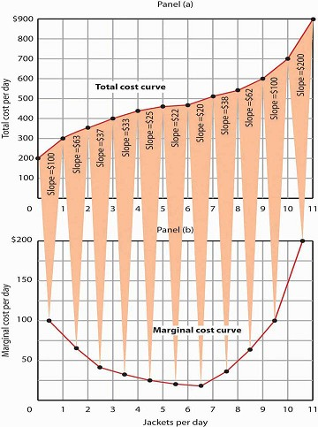
Cost Marginal cost in Panel (b) is the slope of the total cost curve in Panel (a).
Figure 8.7 shows the computation of Acme’s short-run average total cost, average variable cost, and average fixed cost and graphs of these values. Notice that the curves for short-run average total cost and average variable cost fall, then rise. We say that these cost curves are U-shaped. Average fixed costkeeps falling as output increases. This is because the fixed costs are spread out more and more as output expands; by definition, they do not vary as labor is added. Since average total cost (ATC) is the sum of average variable cost (AVC) and average fixed cost (AFC), i.e.,
EQUATION 8.8
AVC + AFC = ATC
the distance between the ATC and AVC curves keeps getting smaller and smaller as the firm spreads its overhead costs over more and more output.
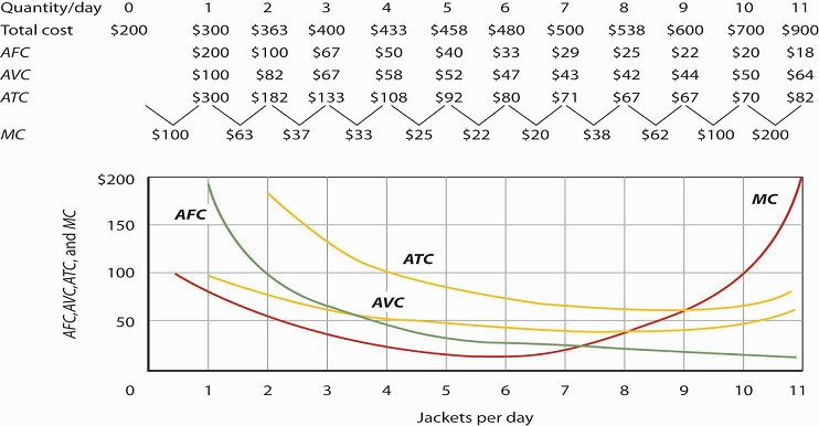
Total cost figures for Acme Clothing are taken from Figure 8.7. The other values are derived from these. Average total cost (ATC) equals total cost divided by quantity produced; it also equals the sum of the average fixed cost (AFC) and average variable cost (AVC) (exceptions in table are due to rounding to the nearest dollar); average variable cost is variable cost divided by quantity produced. The marginal cost (MC) curve (from Figure 8.7) intersects the ATC and AVC curves at the lowest points on both curves. The AFC curve falls as quantity increases.
Figure 8.8 includes the marginal cost data and the marginal cost curve from Figure 8.7. The marginalcost curve intersects the average total cost and average variable cost curves at their lowest points. When marginal cost is below average total cost or average variable cost, the average total and average variable cost curves slope downward. When marginal cost is greater than short-run average total cost or average variable cost, these average cost curves slope upward. The logic behind the relationship between marginalcost and average total and variable costs is the same as it is for the relationship between marginal product and average product.We turn next in this chapter to an examination of production and cost in the long run, a planning period in which the firm can consider changing the quantities of any or all factors.
KEY TAKEAWAYS
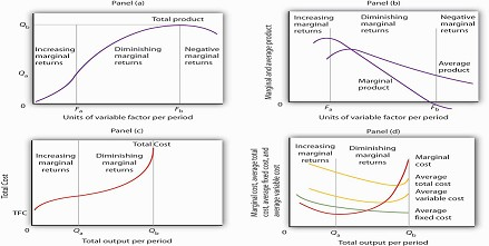
- In Panel (a), the total product curve for a variable factor in the short run shows that the firm experiences increasing marginal returns from zero to Fa units of the variable factor (zero to Qa units of output), diminishing marginal returns from Fa to Fb (Qa to Qb units of output), and negative marginal returns beyond Fb units of the variable factor.
- Panel (b) shows that marginal product rises over the range of increasing marginal returns, falls over the range of diminishing marginal returns, and becomes negative over the range of negative marginal returns. Average product rises when marginal product is above it and falls when marginal product is below it.
- In Panel (c), total cost rises at a decreasing rate over the range of output from zero to Qa This was the range of output that was shown in Panel (a) to exhibit increasing marginal returns. Beyond Qa, the range of diminishing marginal returns, total cost rises at an increasing rate. The total cost at zero units of output(shown as the intercept on the vertical axis) is total fixed cost.
- Panel (d) shows that marginal cost falls over the range of increasing marginal returns, then rises over the range of diminishing marginal returns. The marginal cost curve intersects the average total cost and average variable cost curves at their lowest points. Average fixed cost falls as output increases. Note that average total cost equals average variable cost plus average fixed cost.
- Assuming labor is the variable factor of production, the following definitions and relations describe production and cost in the short run:
- MPL = ΔQ / ΔL
- APL = Q / L
- TVC + TFC = TC
- ATC = TC / Q
- AVC = TVC / Q
- AFC = TFC / Q
- MC = ΔTC / ΔQ
TRY IT!
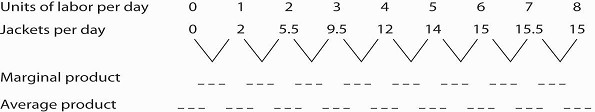
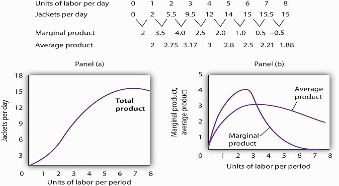
- Suppose Acme gets some new equipment for producing jackets. The table below gives its newproduction function. Compute marginal product and average product and fill in the bottom two rows of the table. Referring to Figure Figure 8.2, draw a graph showing Acme’s new total product curve. On a second graph, below the one showing the total product curve you drew, sketch the marginal and average product curves. Remember to plot marginal product at the midpoint between each input level. On both graphs, shade the regions where Acme experiences increasing marginal returns, diminishing
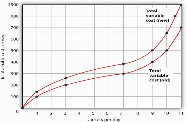
- Draw the points showing total variable cost at daily outputs of 0, 1, 3, 7, 9, 10, and 11 jackets per day when Acme faced a wage of $100 per day. (Use Figure Figure 8.5 as a model.) Sketch the total variable cost curve as shown in Figure Figure 8.4. Now suppose that the wage rises to $125 per day. On the same graph, show the new points and sketch the new total variable cost curve. Explain what has happened. What will happen to Acme’s marginal cost curve? Its average total, average variable, and average fixed cost curves? Explain.
Case in Point: The Production of Fitness
How much should an athlete train?
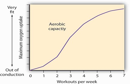
Sports physiologists often measure the “total product” of training as the increase in an athlete’s aerobic capacity—the capacity to absorb oxygen into the bloodstream. An athlete can be
thought of as producing aerobic capacity using a fixed factor (his or her natural capacity) and a variable input (exercise). The chart shows how this aerobic capacity varies with the number
of workouts per week. The curve has a shape very much like a total product curve—which, after all, is precisely what it is. The data suggest that an athlete experiences increasing marginal
returns from exercise for the first three days of training each week; indeed, over half the total gain in aerobic capacity possible is achieved. A person can become even more fit by
exercising more, but the gains become smaller with each added day of training. The law of diminishing marginal returns applies to training.
The increase in fitness that results from the sixth and seventh workouts each week is small. Studies also showthat the costs of daily training, in terms of increased likelihood of injury, are
high. Many trainers and coaches now recommend that athletes—at all levels of competition—take a day or two off each week.
Source: Jeff Galloway, Galloway’s Book on Running (Bolinas, CA: Shelter Publications, 2002), p. 56.
ANSWERS TO TRY IT ! PROBLEMS
- The increased wage will shift the total variable cost curve upward; the old and new points and the corresponding curves are shown at the right.
- The total variable cost curve has shifted upward because the cost of labor, Acme’s variable factor, has increased. The marginal cost curve shows the additional cost of each additional unit of output a firm produces. Because an increase in output requires more labor, and because labor now costs more, the marginal cost curve will shift upward. The increase in total variable cost will increase total cost; average total and average variable costs will rise as well. Average fixed cost will not change.
- 7582 reads
