


Profit-maximizing behavior is always based on the marginal decision rule: Additional units of a good should be produced as long as the marginal revenue of an additional unit exceeds the marginal cost. The maximizing solution occurs where marginal revenue equals marginal cost. As always, firms seek to maximize economic profit, and costs are measured in the economic sense of opportunity cost.
Figure 10.5 shows a demand curve and an associated marginal revenue curve facing a monopoly firm. The marginal cost curve is like those we derived earlier; it falls over the range of output in which the firm experiences increasing marginal returns, then rises as the firm experiences diminishing marginal returns.
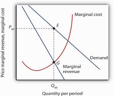
The monopoly firm maximizes profit by producing an output Qm at point G, where the marginal revenue and marginal cost curves intersect. It sells this output at price Pm.
To determine the profit-maximizing output, we note the quantity at which the firm’s marginal revenue and marginal cost curves intersect (Qm in Figure 10.5). We read up from Qm to the demand curve to find the price Pm at which the firm can sell Qm units per period. The profit-maximizing price and output are given by point E on the demand curve.
Thus we can determine a monopoly firm’s profit-maximizing price and output by following three steps:
- Determine the demand, marginal revenue, and marginal cost curves.
- Select the output level at which the marginal revenue and marginal cost curves intersect.
- Determine from the demand curve the price at which that output can be sold.
Once we have determined the monopoly firm’s price and output, we can determine itseconomic profit by adding the firm’s average total cost curve to the graph showing demand, marginal revenue, and marginal cost, as shown in Figure 10.6. The average total cost (ATC) at an output of Qm units is ATCm. The firm’s profit per unit is thus Pm -ATCm. Total profit is found by multiplying the firm’s output, Qm, by profit per unit, so total profit equals Qm(Pm - ATCm)—the area of the shaded rectangle in Figure 10.6.
Heads Up!
Dispelling Myths About Monopoly
Three common misconceptions about monopoly are:
Because there are no rivals selling the products of monopoly firms, they can charge whatever they want. Monopolists will charge whatever the market will bear. Because monopoly firms have the market to themselves, they are guaranteed huge profits.
As Figure 10.5 shows, once the monopoly firm decides on the number of units of output that will maximize profit, the price at which it can sell that many units is found by “reading off” the demand curve the price associated with that many units. If it tries to sell Qm units of output for more than Pm, some of its output will go unsold. The monopoly firm can set its price, but is restricted to price and output combinations that lie on its demand curve. It cannot just “charge whatever it wants.” And if it charges “all the market will bear,” it will sell either 0 or, at most, 1 unit of output.
Neither is the monopoly firm guaranteed a profit. Consider Figure 10.6. Suppose the average total cost curve, instead of lying below the demand curve for some output levels as shown, were instead everywhere above the demand curve. In that case, the monopoly will incur losses no matter what price it chooses, since average total cost will always be greater than any price it might charge. As is the case for perfect competition, the monopoly firm can keep producing in the short run so long as price exceeds average variable cost. In the long run, it will stay in business only if it can cover all of its costs.
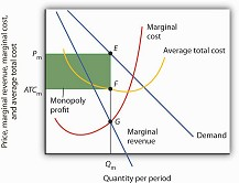
A monopoly firm’s profit per unit is the difference between price and average total cost. Total profit equals profit per unit times the quantity produced. Total profit is given by the area of the shaded rectangle ATCmPmEF.
KEY TAKEAWAYS
- If a firm faces a downward-sloping demand curve, marginal revenue is less than price.
- Marginal revenue is positive in the elastic range of a demand curve, negative in the inelastic range, and zero where demand is unit price elastic.
- If a monopoly firm faces a linear demand curve, its marginal revenue curve is also linear, lies below the demand curve, and bisects any horizontal line drawn from the vertical axis to the demand curve.
- To maximize profit or minimize losses, a monopoly firm produces the quantity at which marginal cost equals marginal revenue. Its price is given by the point on the demand curve that corresponds to this quantity.
TRY IT!
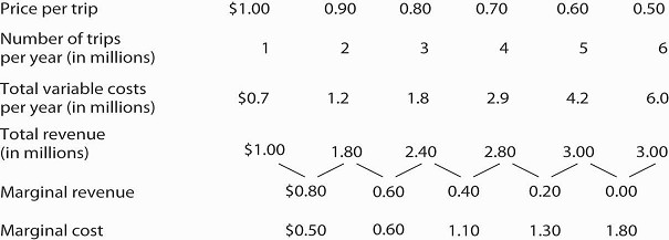
The Troll Road Company is considering building a toll road. It estimates that its linear demand curve is as shown below. Assume that the fixed cost of the road is $0.5 million per year. Maintenance costs, which are the only other costs of the road, are also given in the table.
|
Tolls per trip |
$1.00 |
0.90 |
0.80 |
0.70 |
0.60 |
0.50 |
|---|---|---|---|---|---|---|
|
Number of trips per year (in millions) |
1 |
2 |
3 |
4 |
5 |
6 |
|
Maintenance cost per year (in millions) |
$0.7 |
1.2 |
1.8 |
2.9 |
4.2 |
6.0 |
- Using the midpoint convention, compute the profit-maximizing level of output.
- Using the midpoint convention, what price will the company charge?
- What is marginal revenue at the profit-maximizing output level? How does marginal revenue compare to price?
Case in Point: Profit-Maximizing Hockey Teams
Love of the game? Love of the city? Are those the factors that influence owners of professional sports teams in setting admissions prices? Four economists at the University of Vancouver have
what they think is the answer for one group of teams: professional hockey teams set admission prices at levels that maximize their profits. They regard hockey teams as monopoly firms and use
the monopoly model to examine the team’s behavior.
The economists, Donald G. Ferguson, Kenneth G. Stewart, John Colin H. Jones, and Andre Le Dressay, used data from three seasons to estimate demand and marginal revenue curves facing each team
in the National Hockey League. They found that demand for a team’s tickets is affected by population and income in the team’s home city, the team’s standing in the National Hockey League, and
the number of superstars on the team.
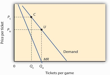
Because a sports team’s costs do not vary significantly with the number of fans who attend a given game, the economists assumed that marginal cost is zero. The profit-maximizing number of
seats sold per game is thus the quantity at which marginal revenue is zero, provided a team’s stadium is large enough to hold that quantity of fans. This unconstrained quantity is labeled Qu,
with a corresponding price Pu in the graph.
Stadium size and the demand curve facing a team might prevent the team from selling the profit-maximizing quantity of tickets. If its stadium holds only Qc fans, for example, the team will
sell that many tickets at price Pc; its marginal revenue is positive at that quantity. Economic theory thus predicts that the marginal revenue for teams that consistently sell out their games
will be positive, and the marginal revenue for other teams will be zero.
The economists’ statistical results were consistent with the theory. They found that teams that don’t typically sell out their games operate at a quantity at which marginal revenue is about
zero, and that teams with sellouts have positive marginal revenue. “It’s clear that these teams are very sophisticated in their use of pricing to maximize profits,” Mr. Ferguson said.
Sources: Donald G. Ferguson et al., “The Pricing of Sports Events: Do Teams Maximize Profit?” Journal of Industrial Economics 39(3) (March 1991): 297–310 and personal interview.
ANSWER TO TRY IT ! PROBLEM
Maintenance costs constitute the variable costs associated with building the road. In order to answer the first four parts of the question, you will need to compute total revenue, marginal revenue, and marginal cost, as shown at right:
- Using the “midpoint” convention, the profit-maximizing level of output is 2.5 million trips per year. With that number of trips, marginal revenue ($0.60) equals marginal cost ($0.60).
- Again, we use the “midpoint” convention. The company will charge a toll of $0.85.
- The marginal revenue is $0.60, which is less than the $0.85 toll (price).
- 10004 reads
