


A demand curve for emitting pollutants shows the quantity of emissions demanded per unit of time at each price. It can, as we have seen, be taken as a marginal benefit curve for emitting pollutants.
The general approach to estimating demand curves involves observing quantities demanded at various prices, together with the values of other determinants of demand. In most pollution problems, however, the price charged for emitting pollutants has always been zero—we simply do not know how the quantity of emissions demanded will vary with price.
One approach to estimating the demand curve for pollution utilizes the fact that this demand occurs because pollution makes other activities cheaper. If we know how much the emission of one more nit of a pollutant saves, then we can infer how much consumers or firms would pay to dump it.
Suppose, for example, that there is no program to control automobile emissions—motorists face a price of zero for each unit of pollution their cars emit. Suppose that a particular motorist’s car emits an average of 10 pounds of carbon monoxide per week. Its owner could reduce emissions to 9 pounds per week at a cost of $1 per week. This $1 is the marginal cost of reducing emissions from 10 to 9 pounds per week. It is also the maximum price the motorist would pay to increase emissions from 9 to 10 pounds per week—it is the marginal benefit of the 10th pound of pollution. We say that it is the maximum price because if asked to pay more, the motorist would choose to reduce emissions at a cost of $1 instead.
Now suppose that emissions have been reduced to 9 pounds per week and that the motorist could reduce them to 8 at an additional cost of $2 per week. The marginal cost of reducing emissions from 9 to 8 pounds per week is $2. Alternatively, this is the maximum price the motorist would be willing to pay to increase emissions to 9 from 8 pounds; it is the marginal benefit of the 9th pound of pollution.Again, if asked to pay more than $2, the motorist would choose to reduce emissions to 8 pounds per week instead.
We can thus think of the marginal benefit of an additional unit of pollution as the added cost of not emitting it. It is the saving a polluter enjoys by dumping additional pollution rather than paying the cost of preventing its emission. Figure 18.2 shows this dual interpretation of cost and benefit. Initially, our motorist emits 10 pounds of carbon monoxide per week. Reading from right to left, the curve measures the marginal costs of pollution abatement (MCA). We see that the marginal cost of abatement rises as emissions are reduced. That makes sense; the first reductions in emissions will be achieved through relatively simple measures such as modifying one’s driving technique to minimize emissions (such as accelerating more slowly), or getting tune-ups more often. Further reductions, however, might require burning more expensive fuels or installing more expensive pollution-control equipment.
Read from left to right, the curve in Figure 18.2 shows the marginal benefit of additional emissions (MBE). Its negative slope suggests that the first units of pollution emitted have very high marginal benefits, because the cost of not emitting them would be very high. As more of a pollutant is emitted, however, its marginal benefit falls—the cost of preventing these units of pollution becomes quite low.
Economists have also measured demand curves for emissions by using surveys in which polluters are asked to report the costs to them of reducing their emissions. In cases in which polluters are charged for the emissions they create, the marginal benefit curve can be observed directly.
As we saw in Figure 18.1, the marginal benefit curves of individual polluters are added horizontally to obtain a market demand curve for pollution. This curve measures the additional benefit to society of each additional unit of pollution.
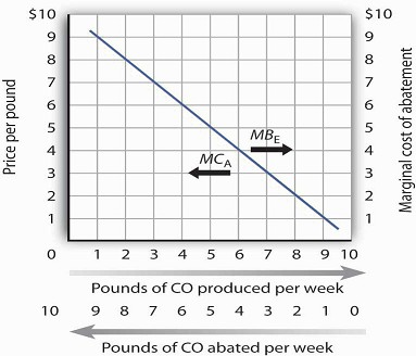
A car emits an average of 10 pounds of CO per week when no restrictions are imposed—when the price of emissions is zero. The marginal cost of abatement (MCA) is the cost of eliminating a unit of emissions; this is the interpretation of the curve when read from right to left. The same curve can be read from left to right as the marginal benefit of emissions (MBE).
Benefits: The Demand for Emissions
- 2902 reads
