


We will use the implicit price deflator as our measure of the price level; the aggregate quantity of goods and services demanded is measured as real GDP. The table in Figure 22.1 gives values for each component of aggregate demand at each price level for a hypothetical economy. Various points on the aggregate demand curve are found by adding the values of these components at different price levels. The aggregate demand curve for the data given in the table is plotted on the graph in Figure 22.1. At point A, at a price level of 1.18, $11,800 billion worth of goods and services will be demanded; at point C, a reduction in the price level to 1.14 increases the quantity of goods and services demanded to $12,000 billion; and at point E, at a price level of 1.10, $12,200 billion will be demanded.
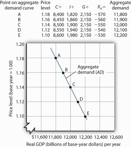
An aggregate demand curve (AD) shows the relationship between the total quantity of output demanded (measured as real GDP) and the price level (measured as the implicit price deflator). At each price level, the total quantity of goods and services demanded is the sum of the components of real GDP, as shown in the table. There is a negative relationship between the price level and the total quantity of goods and services demanded, all other things unchanged.
The negative slope of the aggregate demand curve suggests that it behaves in the same manner as an ordinary demand curve. But we cannot apply the reasoning we use to explain downward-sloping demand curves in individual markets to explain the downward-sloping aggregate demand curve. There are two reasons for a negative relationship between price and quantity demanded in individual markets. First, a lower price induces people to substitute more of the good whose price has fallen for other goods, increasing the quantity demanded. Second, the lower price creates a higher real income. This normally increases quantity demanded further.
Neither of these effects is relevant to a change in prices in the aggregate. When we are dealing with the average of all prices—the price level—we can no longer say that a fall in prices will induce a change in relative prices that will lead consumers to buy more of the goods and services whose prices have fallen and less of the goods and services whose prices have not fallen. The price of corn may have fallen,but the prices of wheat, sugar, tractors, steel, and most other goods or services produced in the economy are likely to have fallen as well.
Furthermore, a reduction in the price level means that it is not just the prices consumers pay that are falling. It means the prices people receive—their wages, the rents they may charge as landlords, the interest rates they earn—are likely to be falling as well. A falling price level means that goods and services are cheaper, but incomes are lower, too. There is no reason to expect that a change in real income will boost the quantity of goods and services demanded—indeed, no change in real income would occur. If nominal incomes and prices all fall by 10%, for example, real incomes do not change.
Why, then, does the aggregate demand curve slope downward? One reason for the downward slope of the aggregate demand curve lies in the relationship between real wealth (the stocks, bonds, and other assets that people have accumulated) and consumption (one of the four components of aggregate demand). When the price level falls, the real value of wealth increases—it packs more purchasing power. For example, if the price level falls by 25%, then $10,000 of wealth could purchase more goods and services than it would have if the price level had not fallen. An increase in wealth will induce people to increase their consumption. The consumption component of aggregate demand will thus be greater at lower price levels than at higher price levels. The tendency for a change in the price level to affect real wealth and thus alter consumption is called the wealth effect; it suggests a negative relationship between the price level and the real value of consumption spending.
A second reason the aggregate demand curve slopes downward lies in the relationship between interest rates and investment. A lower price level lowers the demand for money, because less money is required to buy a given quantity of goods. What economists mean by money demand will be explained in more detail in a later chapter. But, as we learned in studying demand and supply, a reduction in the demand for something, all other things unchanged, lowers its price. In this case, the “something” is money and its price is the interest rate. A lower price level thus reduces interest rates. Lower interest rates make borrowing by firms to build factories or buy equipment and other capital more attractive. A lower interest rate means lower mortgage payments, which tends to increase investment in residential houses. Investment thus rises when the price level falls. The tendency for a change in the price level to affect the interest rate and thus to affect the quantity of investment demanded is called the interest rate effect. John Maynard Keynes, a British economist whose analysis of the Great Depression and what to do about it led to the birth of modern macroeconomics, emphasized this effect. For this reason, the interest rate effect is sometimes called the Keynes effect.
A third reason for the rise in the total quantity of goods and services demanded as the price level falls can be found in changes in the net export component of aggregate demand. All other things unchanged, a lower price level in an economy reduces the prices of its goods and services relative to foreign-produced goods and services. A lower price level makes that economy’s goods more attractive to foreign buyers, increasing exports. It will also make foreign-produced goods and services less attractive to the economy’s buyers, reducing imports. The result is an increase in net exports. The international trade effect is the tendency for a change in the price level to affect net exports.
Taken together, then, a fall in the price level means that the quantities of consumption, investment,and net export components of aggregate demand may all rise. Since government purchases are determined through a political process, we assume there is no causal link between the price level and the real volume of government purchases. Therefore, this component of GDP does not contribute to the downward slope of the curve.
In general, a change in the price level, with all other determinants of aggregate demand unchanged,causes a movement along the aggregate demand curve. A movement along an aggregate demand curve is a change in the aggregate quantity of goods and services demanded. A movement from point A to point B on the aggregate demand curve in Figure 22.1 is an example. Such a change is a response to a change in the price level.
Notice that the axes of the aggregate demand curve graph are drawn with a break near the origin to remind us that the plotted values reflect a relatively narrow range of changes in real GDP and the price level. We do not know what might happen if the price level or output for an entire economy approached zero. Such a phenomenon has never been observed.
- 9330 reads
