


Real GDP is a measure of the total output of firms. Aggregate expenditures equal total planned spending on that output. Equilibrium in the model occurs where aggregate expenditures in some period equal real GDP in that period. One way to think about equilibrium is to recognize that firms, except for some inventory that they plan to hold, produce goods and services with the intention of selling them. Aggregate expenditures consist of what people, firms, and government agencies plan to spend. If the economy is at its equilibrium real GDP, then firms are selling what they plan to sell (that is, there are no unplanned changes in inventories).
Figure 28.8 illustrates the concept of equilibrium in the aggregate expenditures model. A 45-degree line connects all the points at which the values on the two axes, representing aggregate expenditures and real GDP, are equal. Equilibrium must occur at some point along this 45-degree line. The point at which the aggregate expenditures curve crosses the 45-degree line is the equilibrium real GDP, here achieved at a real GDP of $7,000 billion.
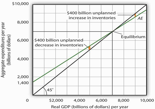
Equation 28.11 tells us that at a real GDP of $7,000 billion, the sum of consumption and planned investment is $7,000 billion—precisely the level of output firms produced. At that level of output, firms sell what they planned to sell and keep inventories that they planned to keep. A real GDP of $7,000 billion represents equilibrium in the sense that it generates an equal level of aggregate expenditures.
If firms were to produce a real GDP greater than $7,000 billion per year, aggregate expenditures would fall short of real GDP. At a level of real GDP of $9,000 billion per year, for example, aggregate expenditures equal $8,600 billion. Firms would be left with $400 billion worth of goods they intended to sell but did not. Their actual level of investment would be $400 billion greater than their planned level of investment. With those unsold goods on hand (that is, with an unplanned increase in inventories), firms would be likely to cut their output, moving the economy toward its equilibrium GDP of $7,000 billion. If firms were to produce $5,000 billion, aggregate expenditures would be $5,400 billion. Consumers and firms would demand more than was produced; firms would respond by reducing their inventories below the planned level (that is, there would be an unplanned decrease in inventories) and increasing their output in subsequent periods, again moving the economy toward its equilibrium real GDP of $7,000 billion. Figure 28.9 shows possible levels of real GDP in the economy for the aggregate expenditures function illustrated in Figure 28.8. It shows the level of aggregate expenditures at various levels of real GDP and the direction in which real GDP will change whenever AE does not equal real GDP. At any level of real GDP other than the equilibrium level, there is unplanned investment.
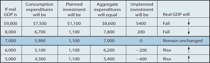
Each level of real GDP will result in a particular amount of aggregate expenditures. If aggregate expenditures are less than the level of real GDP, firms will reduce their output and real GDP will fall. If aggregate expenditures exceed real GDP, then firms will increase their output and real GDP will rise. If aggregate expenditures equal real GDP, then firms will leave their output unchanged; we have achieved equilibrium in the aggregate expenditures model. At equilibrium, there is no unplanned investment. Here, that occurs at a real GDP of $7,000 billion.
- 6998 reads
