


The scaling of the vertical axis in time-series graphs can give very different views of economic data. We can make a variable appear to change a great deal, or almost not at all, depending on how we scale the axis. For that reason, it is important to note carefully how the vertical axis in a time-series graph is scaled.
Consider, for example, the issue of whether an increase or decrease in income tax rates has a significant effect on federal government revenues. This became a big issue in 1993, when President Clinton proposed an increase in income tax rates. The measure was intended to boost federal revenues. Critics of the president’s proposal argued that changes in tax rates have little or no effect on federal revenues. Higher tax rates, they said, would cause some people to scale back their income-earning efforts and thus produce only a small gain—or even a loss—in revenues. Op-ed essays in The Wall Street Journal, for example, often showed a graph very much like that presented in Panel (a) of Figure 20.21. It shows federal revenues as a percentage of gross domestic product (GDP), a measure of total income in the economy, since 1960. Various tax reductions and increases were enacted during that period, but Panel (a) appears to show they had little effect on federal revenues relative to total income.
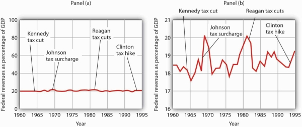
A graph of federal revenues as a percentage of GDP emphasizes the stability of the relationship when plotted with the vertical axis scaled from 0 to 100, as in Panel (a). Scaling the vertical axis from 16 to 21%, as in Panel (b), stresses the short-term variability of the percentage and suggests that major tax rate changes have affected federal revenues.
Laura Tyson, then President Clinton’s chief economic adviser, charged that those graphs were misleading. In a Wall Street Journal piece, she noted the scaling of the vertical axis used by the president’s critics. She argued that a more reasonable scaling of the axis shows that federal revenues tend to increase relative to total income in the economy and that cuts in taxes reduce the federal government’s share. Her alternative version of these events does, indeed, suggest that federal receipts have tended to rise and fall with changes in tax policy, as shown in Panel (b) of Figure 20.21.
Which version is correct? Both are. Both graphs show the same data. It is certainly true that federal revenues, relative to economic activity, have been remarkably stable over the past several decades, as emphasized by the scaling in Panel (a). But it is also true that the federal share has varied between about 17 and 20%. And a small change in the federal share translates into a large amount of tax revenue.
It is easy to be misled by time-series graphs. Large changes can be made to appear trivial and trivial changes to appear large through an artful scaling of the axes. The best advice for a careful consumer of graphical information is to note carefully the range of values shown and then to decide whether the changes are really significant.
- 1301 reads
